Note
Click here to download the full example code
Slope estimation via Structure Tensor algorithm
This example shows how to estimate local slopes of a two-dimensional array
using pylops.utils.signalprocessing.slope_estimate.
Knowing the local slopes of an image (or a seismic data) can be useful for
a variety of tasks in image (or geophysical) processing such as denoising,
smoothing, or interpolation. When slopes are used with the
pylops.signalprocessing.Seislet operator, the input dataset can be
compressed and the sparse nature of the Seislet transform can also be used to
precondition sparsity-promoting inverse problems.
import numpy as np
import matplotlib.pyplot as plt
from scipy.ndimage import gaussian_filter

import pylops
from pylops.signalprocessing.Seislet import _predict_trace

plt.close('all')
np.random.seed(10)
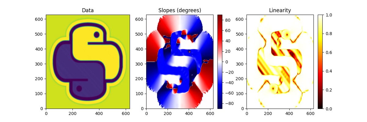
To start we import a 2d image and estimate the local slopes of the image.
im = np.load('../testdata/python.npy')[..., 0]
im = im / 255. - 0.5
im = gaussian_filter(im, sigma=2)

slopes, linearity = \
    pylops.utils.signalprocessing.slope_estimate(im, 1., 1., smooth=7)

fig, axs = plt.subplots(1, 3, figsize=(12, 4))
iax = axs[0].imshow(im, cmap='viridis', origin='lower')
axs[0].set_title('Data')
axs[0].axis('tight')
iax = axs[1].imshow(-np.rad2deg(slopes), cmap='seismic', origin='lower',
                    vmin=-90, vmax=90)
axs[1].set_title('Slopes (degrees)')
plt.colorbar(iax, ax=axs[1])
axs[1].axis('tight')
iax = axs[2].imshow(linearity, cmap='hot', origin='lower', vmin=0, vmax=1)
axs[2].set_title('Linearity')
plt.colorbar(iax, ax=axs[2])
axs[2].axis('tight')
Out:
(-0.5, 629.5, -0.5, 629.5)
We can now repeat the same using some seismic data. We will first define a single trace and a slope field, apply such slope field to the trace recursively to create the other traces of the data and finally try to recover the underlying slope field from the data alone.
# Reflectivity model
nx, nt = 2**7, 121
dx, dt = 4, 0.004
x, t = np.arange(nx)*dx, np.arange(nt)*dt

refl = np.zeros(nt)
it = np.sort(np.random.permutation(np.arange(10, nt-20))[:nt//8])
refl[it] = np.random.normal(0., 1., nt//8)

# Wavelet
ntwav = 41
f0 = 30
wav = pylops.utils.wavelets.ricker(np.arange(ntwav)*0.004, f0)[0]
wavc = np.argmax(wav)

# Input trace
trace = np.convolve(refl, wav, mode='same')

# Slopes
theta = np.linspace(0, 30, nx)
slope = np.outer(np.ones(nt), np.deg2rad(theta) * dt / dx)

# Model data
d = np.zeros((nt, nx))
tr = trace.copy()
for ix in range(nx):
    tr = _predict_trace(tr, t, dt, dx, slope[:, ix])
    d[:, ix] = tr

# Estimate slopes
slope_est = -pylops.utils.signalprocessing.slope_estimate(d, dt, dx,
                                                          smooth=10)[0]

fig, axs = plt.subplots(1, 3, figsize=(12, 5))
axs[0].imshow(d, cmap='gray', vmin=-1, vmax=1,
              extent=(x[0], x[-1], t[-1], t[0]))
axs[0].set_title('Data')
axs[0].axis('tight')
axs[1].imshow(np.rad2deg(slope)*dx/dt, cmap='seismic', vmin=0, vmax=40,
              extent=(x[0], x[-1], t[-1], t[0]))
axs[1].set_title('True Slopes')
axs[1].axis('tight')
iax = axs[2].imshow(np.rad2deg(slope_est)*dx/dt, cmap='seismic',
                    vmin=0, vmax=40,
                    extent=(x[0], x[-1], t[-1], t[0]))
axs[2].set_title('Estimated Slopes')
plt.colorbar(iax, ax=axs[2])
axs[2].axis('tight')
Out:
(0.0, 508.0, 0.48, 0.0)
As you can see the Structure Tensor algorithm is a very fast, general purpose algorithm that can be used to estimate local slopes to input datasets of very different nature.
Total running time of the script: ( 0 minutes 7.611 seconds)