Note
Click here to download the full example code
Wavelet transform
This example shows how to use the pylops.DWT and
pylops.DWT2D operators to perform 1- and 2-dimensional DWT.
import numpy as np
import matplotlib.pyplot as plt

import pylops

plt.close('all')
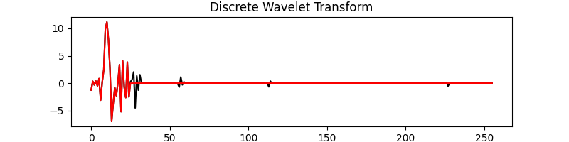
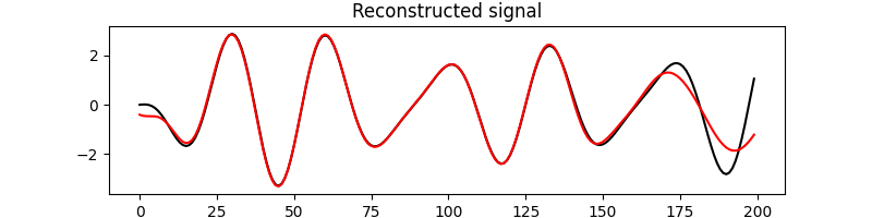
Let’s start with a 1-dimensional signal. We apply the 1-dimensional wavelet transform, keep only the first 30 coefficients and perform the inverse transform.
nt = 200
dt = 0.004
t = np.arange(nt)*dt
freqs = [10, 7, 9]
amps = [1, -2, .5]
x = np.sum([amp * np.sin(2 * np.pi * f * t) for (f, amp) in zip(freqs, amps)], axis=0)

Wop = pylops.signalprocessing.DWT(nt, wavelet='dmey', level=5)
y = Wop * x
yf = y.copy()
yf[25:] = 0
xinv = Wop.H * yf

plt.figure(figsize=(8,2))
plt.plot(y, 'k', label='Full')
plt.plot(yf, 'r', label='Extracted')
plt.title('Discrete Wavelet Transform')

plt.figure(figsize=(8,2))
plt.plot(x, 'k', label='Original')
plt.plot(xinv, 'r', label='Reconstructed')
plt.title('Reconstructed signal')
Out:
Text(0.5, 1.0, 'Reconstructed signal')
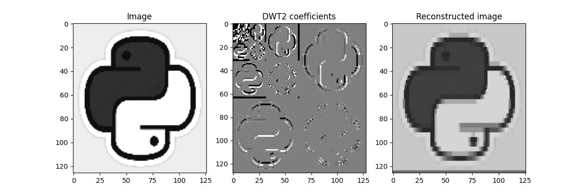
We repeat the same procedure with an image. In this case the 2-dimensional DWT will be applied instead. Only a quarter of the coefficients of the DWT will be retained in this case.
im = np.load('../testdata/python.npy')[::5, ::5, 0]

Nz, Nx = im.shape
Wop = pylops.signalprocessing.DWT2D((Nz, Nx), wavelet='haar', level=5)
y = Wop * im.ravel()
yf = y.copy()
yf[len(y)//4:] = 0
iminv = Wop.H * yf
iminv = iminv.reshape(Nz, Nx)

fig, axs = plt.subplots(1, 3, figsize=(12, 4))
axs[0].imshow(im, cmap='gray')
axs[0].set_title('Image')
axs[0].axis('tight')
axs[1].imshow(y.reshape(Wop.dimsd), cmap='gray_r', vmin=-1e2, vmax=1e2)
axs[1].set_title('DWT2 coefficients')
axs[1].axis('tight')
axs[2].imshow(iminv, cmap='gray')
axs[2].set_title('Reconstructed image')
axs[2].axis('tight')
Out:
(-0.5, 125.5, 125.5, -0.5)
Total running time of the script: ( 0 minutes 0.456 seconds)