pylops.waveeqprocessing.PhaseShift
-
pylops.waveeqprocessing.PhaseShift(vel, dz, nt, freq, kx, ky=None, dtype='float64')[source]¶ Phase shift operator
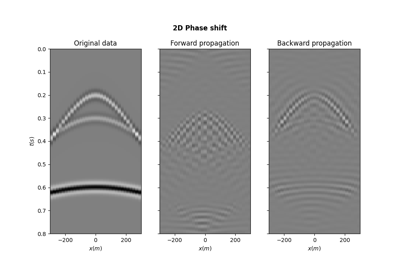
Apply positive (forward) phase shift with constant velocity in forward mode, and negative (backward) phase shift with constant velocity in adjoint mode. Input model and data should be 2- or 3-dimensional arrays in time-space domain of size \([n_t \times n_x \;(\times n_y)]\).
Parameters: - vel :
float, optional Constant propagation velocity
- dz :
float, optional Depth step
- nt :
int, optional Number of time samples of model and data
- freq :
numpy.ndarray Positive frequency axis
- kx :
int, optional Horizontal wavenumber axis (centered around 0) of size \([n_x \times 1]\).
- ky :
int, optional Second horizontal wavenumber axis for 3d phase shift (centered around 0) of size \([n_y \times 1]\).
- dtype :
str, optional Type of elements in input array
Returns: - Pop :
pylops.LinearOperator Phase shift operator
Notes
The phase shift operator implements a one-way wave equation forward propagation in frequency-wavenumber domain by applying the following transformation to the input model:
\[d(f, k_x, k_y) = m(f, k_x, k_y) e^{-j \Delta z \sqrt{\omega^2/v^2 - k_x^2 - k_y^2}}\]where \(v\) is the constant propagation velocity and \(\Delta z\) is the propagation depth. In adjoint mode, the data is propagated backward using the following transformation:
\[m(f, k_x, k_y) = d(f, k_x, k_y) e^{j \Delta z \sqrt{\omega^2/v^2 - k_x^2 - k_y^2}}\]Effectively, the input model and data are assumed to be in time-space domain and forward Fourier transform is applied to both dimensions, leading to the following operator:
\[\mathbf{d} = \mathbf{F}^H_t \mathbf{F}^H_x \mathbf{P} \mathbf{F}_x \mathbf{F}_t \mathbf{m}\]where \(\mathbf{P}\) perfoms the phase-shift as discussed above.
- vel :