Restriction and Interpolation

This example shows how to use the pylops.Restriction operator to sample a certain input vector at desired locations iava. Moreover, we go one step further and use the pylops.signalprocessing.Interp operator to show how we can also sample values at locations that are not exactly on the grid of the input vector.

As explained in the 03. Solvers tutorial, such operators can be used as forward model in an inverse problem aimed at interpolate irregularly sampled 1d or 2d signals onto a regular grid.

import matplotlib.pyplot as plt
import numpy as np

import pylops

plt.close("all")
np.random.seed(10)

Let’s create a signal of size nt and sampling dt that is composed of three sinusoids at frequencies freqs.

nt = 200
dt = 0.004

freqs = [5.0, 3.0, 8.0]

t = np.arange(nt) * dt
x = np.zeros(nt)

for freq in freqs:
    x = x + np.sin(2 * np.pi * freq * t)

First of all, we subsample the signal at random locations and we retain 40% of the initial samples.

perc_subsampling = 0.4
ntsub = int(np.round(nt * perc_subsampling))

isample = np.arange(nt)
iava = np.sort(np.random.permutation(np.arange(nt))[:ntsub])

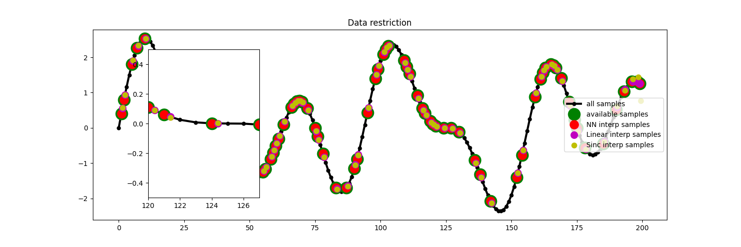
We then create the restriction and interpolation operators and display the original signal as well as the subsampled signal.

Rop = pylops.Restriction(nt, iava, dtype="float64")
NNop, iavann = pylops.signalprocessing.Interp(
    nt, iava + 0.4, kind="nearest", dtype="float64"
)
LIop, iavali = pylops.signalprocessing.Interp(
    nt, iava + 0.4, kind="linear", dtype="float64"
)
SIop, iavasi = pylops.signalprocessing.Interp(
    nt, iava + 0.4, kind="sinc", dtype="float64"
)
y = Rop * x
ynn = NNop * x
yli = LIop * x
ysi = SIop * x
ymask = Rop.mask(x)

# Visualize data
fig = plt.figure(figsize=(15, 5))
plt.plot(isample, x, ".-k", lw=3, ms=10, label="all samples")
plt.plot(isample, ymask, ".g", ms=35, label="available samples")
plt.plot(iavann, ynn, ".r", ms=25, label="NN interp samples")
plt.plot(iavali, yli, ".m", ms=20, label="Linear interp samples")
plt.plot(iavasi, ysi, ".y", ms=15, label="Sinc interp samples")
plt.legend(loc="right")
plt.title("Data restriction")

subax = fig.add_axes([0.2, 0.2, 0.15, 0.6])
subax.plot(isample, x, ".-k", lw=3, ms=10)
subax.plot(isample, ymask, ".g", ms=35)
subax.plot(iavann, ynn, ".r", ms=25)
subax.plot(iavali, yli, ".m", ms=20)
subax.plot(iavasi, ysi, ".y", ms=15)
subax.set_xlim([120, 127])
subax.set_ylim([-0.5, 0.5])

Out:

(-0.5, 0.5)

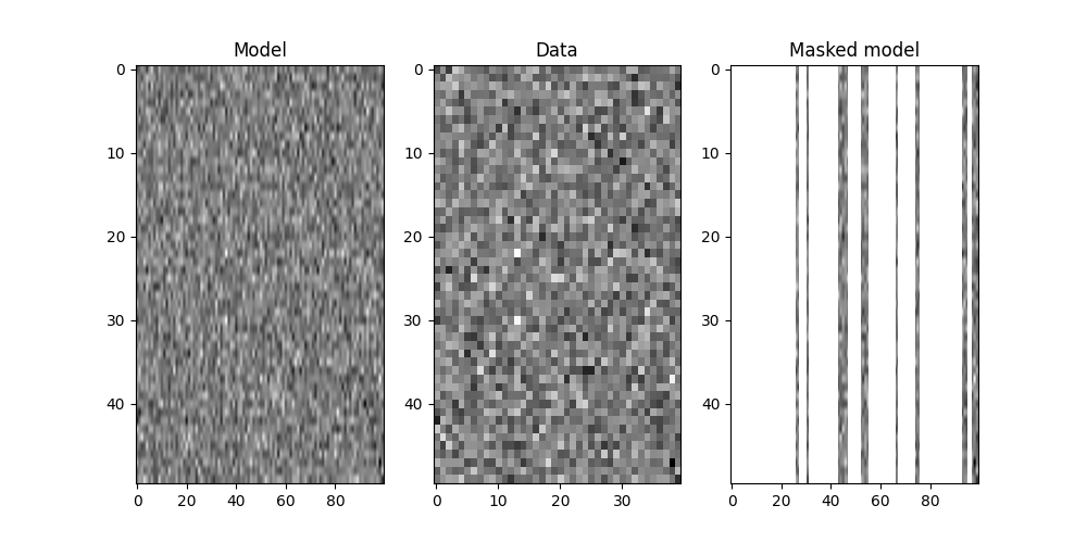
Finally we show how the pylops.Restriction is not limited to one dimensional signals but can be applied to sample locations of a specific axis of a multi-dimensional array. subsampling locations

nx, nt = 100, 50

x = np.random.normal(0, 1, (nx, nt))

perc_subsampling = 0.4
nxsub = int(np.round(nx * perc_subsampling))
iava = np.sort(np.random.permutation(np.arange(nx))[:nxsub])

Rop = pylops.Restriction(nx * nt, iava, dims=(nx, nt), dir=0, dtype="float64")
y = (Rop * x.ravel()).reshape(nxsub, nt)
ymask = Rop.mask(x)

fig, axs = plt.subplots(1, 3, figsize=(10, 5))
axs[0].imshow(x.T, cmap="gray")
axs[0].set_title("Model")
axs[0].axis("tight")
axs[1].imshow(y.T, cmap="gray")
axs[1].set_title("Data")
axs[1].axis("tight")
axs[2].imshow(ymask.T, cmap="gray")
axs[2].set_title("Masked model")
axs[2].axis("tight")

Out:

(-0.5, 99.5, 49.5, -0.5)