Note
Click here to download the full example code
09. Marchenko redatuming by inversion
This example shows how to set-up and run the
pylops.waveeqprocessing.Marchenko inversion using synthetic data.
Let’s start by defining some input parameters and loading the test data
# Input parameters
inputfile = '../testdata/marchenko/input.npz'
vs_zx = [1060, 1200] # virtual source z,x
vel = 2400.0 # velocity
toff = 0.045 # direct arrival time shift
nsmooth = 10 # time window smoothing
nfmax = 1000 # max frequency for MDC (#samples)
niter = 10 # iterations
inputdata = np.load(inputfile)
# Receivers
r = inputdata['r']
nr = r.shape[1]
dr = r[0, 1]-r[0, 0]
# Sources
s = inputdata['s']
ns = s.shape[1]
ds = s[0, 1]-s[0, 0]
# Virtual points
vs = inputdata['vs']
# Density model
rho = inputdata['rho']
z, x = inputdata['z'], inputdata['x']
# Reflection data and subsurface fields
R = inputdata['R'][:, :, :-100]
R = np.swapaxes(R, 0, 1)
Gsub = inputdata['Gsub'][:-100]
G0sub = inputdata['G0sub'][:-100]
wav = inputdata['wav']
wav_c = np.argmax(wav)
t = inputdata['t'][:-100]
ot, dt, nt = t[0], t[1]-t[0], len(t)
Gsub = np.apply_along_axis(convolve, 0, Gsub, wav, mode='full')
Gsub = Gsub[wav_c:][:nt]
G0sub = np.apply_along_axis(convolve, 0, G0sub, wav, mode='full')
G0sub = G0sub[wav_c:][:nt]
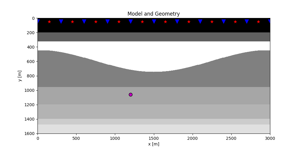
plt.figure(figsize=(10, 5))
plt.imshow(rho, cmap='gray', extent=(x[0], x[-1], z[-1], z[0]))
plt.scatter(s[0, 5::10], s[1, 5::10], marker='*', s=150, c='r', edgecolors='k')
plt.scatter(r[0, ::10], r[1, ::10], marker='v', s=150, c='b', edgecolors='k')
plt.scatter(vs[0], vs[1], marker='.', s=250, c='m', edgecolors='k')
plt.axis('tight')
plt.xlabel('x [m]')
plt.ylabel('y [m]')
plt.title('Model and Geometry')
plt.xlim(x[0], x[-1])
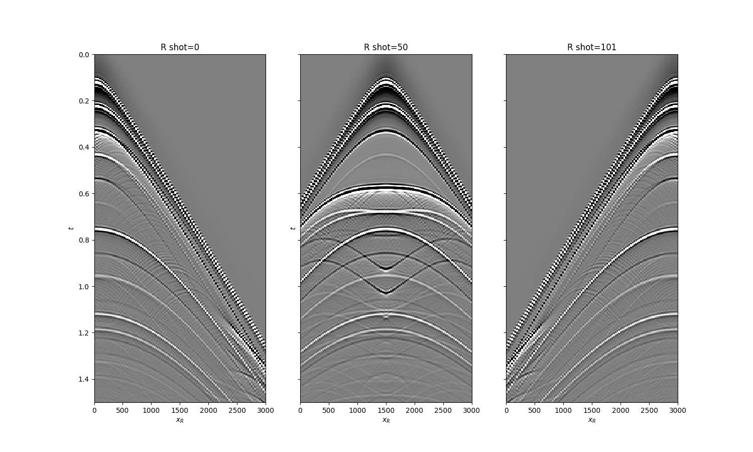
fig, axs = plt.subplots(1, 3, sharey=True, figsize=(15, 9))
axs[0].imshow(R[0].T, cmap='gray', vmin=-1e-2, vmax=1e-2,
extent=(r[0, 0], r[0, -1], t[-1], t[0]))
axs[0].set_title('R shot=0')
axs[0].set_xlabel(r'$x_R$')
axs[0].set_ylabel(r'$t$')
axs[0].axis('tight')
axs[0].set_ylim(1.5, 0)
axs[1].imshow(R[ns//2].T, cmap='gray', vmin=-1e-2, vmax=1e-2,
extent=(r[0, 0], r[0, -1], t[-1], t[0]))
axs[1].set_title('R shot=%d' %(ns//2))
axs[1].set_xlabel(r'$x_R$')
axs[1].set_ylabel(r'$t$')
axs[1].axis('tight')
axs[1].set_ylim(1.5, 0)
axs[2].imshow(R[-1].T, cmap='gray', vmin=-1e-2, vmax=1e-2,
extent=(r[0, 0], r[0, -1], t[-1], t[0]))
axs[2].set_title('R shot=%d' %ns)
axs[2].set_xlabel(r'$x_R$')
axs[2].axis('tight')
axs[2].set_ylim(1.5, 0)
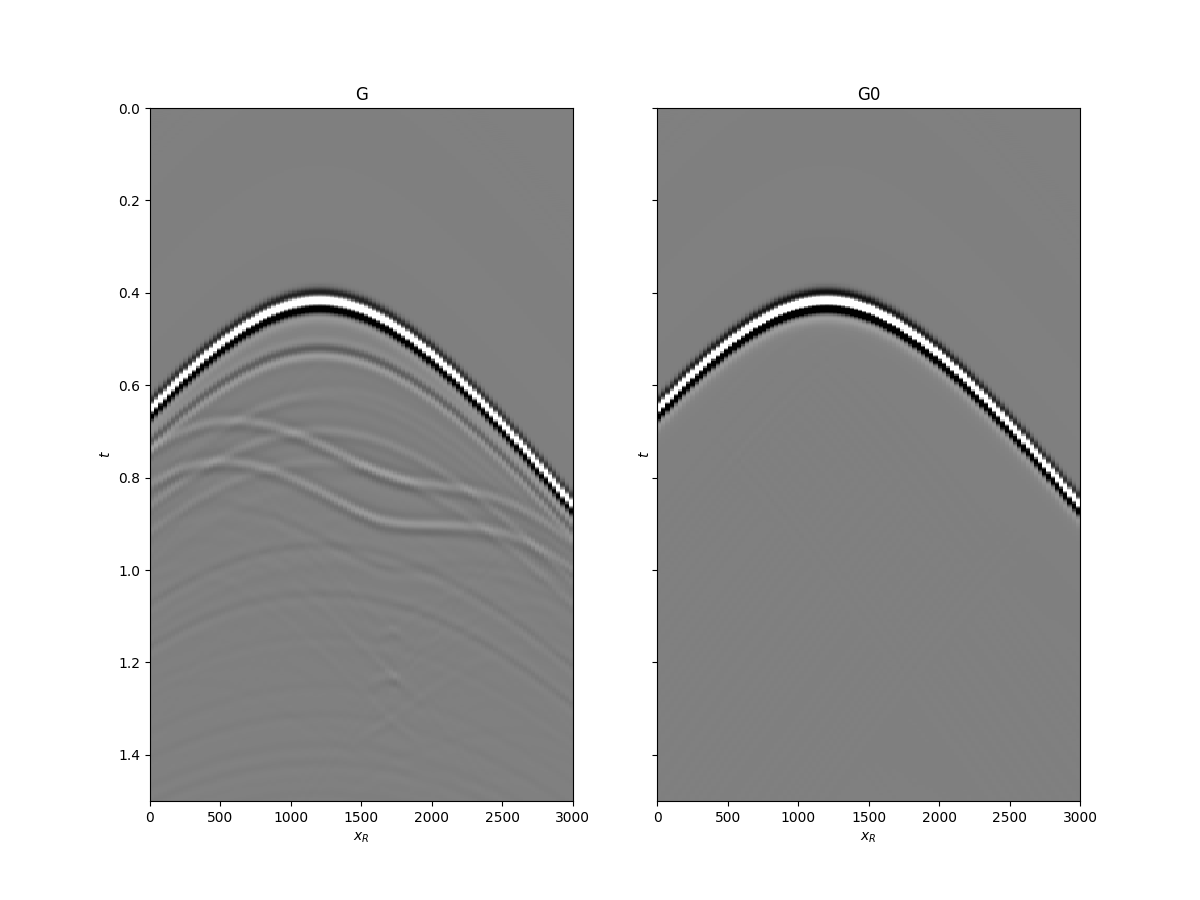
fig, axs = plt.subplots(1, 2, sharey=True, figsize=(12, 9))
axs[0].imshow(Gsub, cmap='gray', vmin=-1e6, vmax=1e6,
extent=(r[0, 0], r[0, -1], t[-1], t[0]))
axs[0].set_title('G')
axs[0].set_xlabel(r'$x_R$')
axs[0].set_ylabel(r'$t$')
axs[0].axis('tight')
axs[0].set_ylim(1.5, 0)
axs[1].imshow(G0sub, cmap='gray', vmin=-1e6, vmax=1e6,
extent=(r[0, 0], r[0, -1], t[-1], t[0]))
axs[1].set_title('G0')
axs[1].set_xlabel(r'$x_R$')
axs[1].set_ylabel(r'$t$')
axs[1].axis('tight')
axs[1].set_ylim(1.5, 0)
Let’s now create an object of the
pylops.waveeqprocessing.Marchenko class and apply redatuming
for a single subsurface point vs.
# direct arrival window
trav = np.sqrt((vs[0]-r[0])**2+(vs[1]-r[1])**2)/vel

MarchenkoWM = Marchenko(R, dt=dt, dr=dr, nfmax=nfmax, wav=wav,
                        toff=toff, nsmooth=nsmooth)

f1_inv_minus, f1_inv_plus, p0_minus, g_inv_minus, g_inv_plus = \
    MarchenkoWM.apply_onepoint(trav, G0=G0sub.T, rtm=True, greens=True,
                               dottest=True, **dict(iter_lim=niter, show=True))
g_inv_tot = g_inv_minus + g_inv_plus
Out:
/home/docs/checkouts/readthedocs.org/user_builds/pylops/envs/v1.5.0/lib/python3.6/site-packages/pylops-1.5.0-py3.6.egg/pylops/waveeqprocessing/marchenko.py:182: FutureWarning: A new implementation of Marchenko is provided in v1.5.0. This currently affects only the inner working of the operator, end-users can continue using the operator in the same way. Nevertheless, R1 is not required anymoreeven when R is provided in frequency domain. It is recommended to start using the operator without the R1 input as this behaviour will become default in version v2.0.0 and R1 will be removed from the inputs.
/home/docs/checkouts/readthedocs.org/user_builds/pylops/envs/v1.5.0/lib/python3.6/site-packages/pylops-1.5.0-py3.6.egg/pylops/waveeqprocessing/mdd.py:112: FutureWarning: A new implementation of MDC is provided in v1.5.0. This currently affects only the inner working of the operator, end-users can continue using the operator in the same way. Nevertheless, it is now recommended to start using the operator with transpose=True, as this behaviour will become default in version v2.0.0 and the behaviour with transpose=False will be deprecated.
/home/docs/checkouts/readthedocs.org/user_builds/pylops/envs/v1.5.0/lib/python3.6/site-packages/pylops-1.5.0-py3.6.egg/pylops/utils/dottest.py:69: ComplexWarning: Casting complex values to real discards the imaginary part
Dot test passed, v^T(Opu)=491.131956 - u^T(Op^Tv)=491.131956
/home/docs/checkouts/readthedocs.org/user_builds/pylops/envs/v1.5.0/lib/python3.6/site-packages/pylops-1.5.0-py3.6.egg/pylops/basicoperators/BlockDiag.py:104: ComplexWarning: Casting complex values to real discards the imaginary part
Dot test passed, v^T(Opu)=464.113195 - u^T(Op^Tv)=464.113195

LSQR            Least-squares solution of  Ax = b
The matrix A has   282598 rows  and   282598 cols
damp = 0.00000000000000e+00   calc_var =        0
atol = 1.00e-08                 conlim = 1.00e+08
btol = 1.00e-08               iter_lim =       10

   Itn      x[0]       r1norm     r2norm   Compatible    LS      Norm A   Cond A
     0  0.00000e+00   3.134e+07  3.134e+07    1.0e+00  3.3e-08
     1  0.00000e+00   1.374e+07  1.374e+07    4.4e-01  9.3e-01   1.1e+00  1.0e+00
     2  0.00000e+00   7.770e+06  7.770e+06    2.5e-01  3.9e-01   1.8e+00  2.2e+00
     3  0.00000e+00   5.750e+06  5.750e+06    1.8e-01  3.3e-01   2.1e+00  3.4e+00
     4  0.00000e+00   3.930e+06  3.930e+06    1.3e-01  3.4e-01   2.5e+00  5.1e+00
     5  0.00000e+00   3.042e+06  3.042e+06    9.7e-02  2.6e-01   2.9e+00  6.8e+00
     6  0.00000e+00   2.423e+06  2.423e+06    7.7e-02  2.2e-01   3.3e+00  8.6e+00
     7  0.00000e+00   1.675e+06  1.675e+06    5.3e-02  2.5e-01   3.6e+00  1.1e+01
     8  0.00000e+00   1.248e+06  1.248e+06    4.0e-02  2.0e-01   3.9e+00  1.3e+01
     9  0.00000e+00   1.004e+06  1.004e+06    3.2e-02  1.5e-01   4.2e+00  1.4e+01
    10  0.00000e+00   7.762e+05  7.762e+05    2.5e-02  1.8e-01   4.4e+00  1.6e+01

LSQR finished
The iteration limit has been reached

istop =       7   r1norm = 7.8e+05   anorm = 4.4e+00   arnorm = 6.1e+05
itn   =      10   r2norm = 7.8e+05   acond = 1.6e+01   xnorm  = 3.6e+07
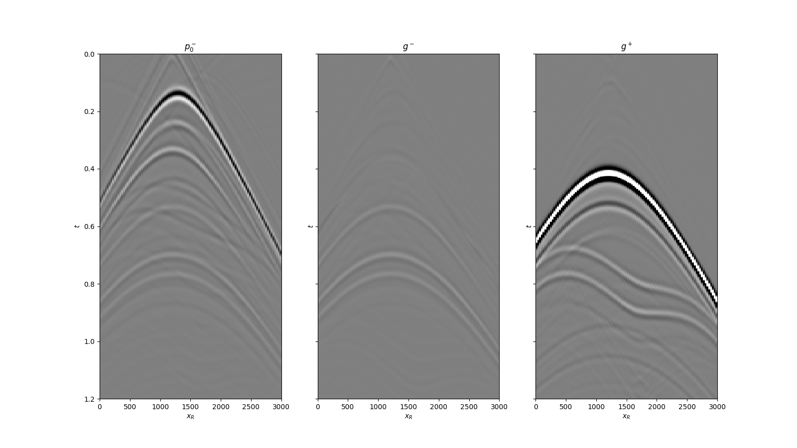
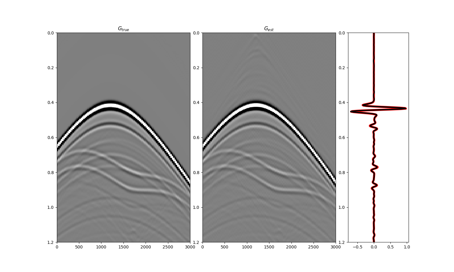
We can now compare the result of Marchenko redatuming via LSQR with standard redatuming
fig, axs = plt.subplots(1, 3, sharey=True, figsize=(16, 9))
axs[0].imshow(p0_minus.T, cmap='gray', vmin=-5e5, vmax=5e5,
              extent=(r[0, 0], r[0, -1], t[-1], -t[-1]))
axs[0].set_title(r'$p_0^-$')
axs[0].set_xlabel(r'$x_R$')
axs[0].set_ylabel(r'$t$')
axs[0].axis('tight')
axs[0].set_ylim(1.2, 0)
axs[1].imshow(g_inv_minus.T, cmap='gray', vmin=-5e5, vmax=5e5,
              extent=(r[0, 0], r[0, -1], t[-1], -t[-1]))
axs[1].set_title(r'$g^-$')
axs[1].set_xlabel(r'$x_R$')
axs[1].set_ylabel(r'$t$')
axs[1].axis('tight')
axs[1].set_ylim(1.2, 0)
axs[2].imshow(g_inv_plus.T, cmap='gray', vmin=-5e5, vmax=5e5,
              extent=(r[0, 0], r[0, -1], t[-1], -t[-1]))
axs[2].set_title(r'$g^+$')
axs[2].set_xlabel(r'$x_R$')
axs[2].set_ylabel(r'$t$')
axs[2].axis('tight')
axs[2].set_ylim(1.2, 0)

fig = plt.figure(figsize=(15, 9))
ax1 = plt.subplot2grid((1, 5), (0, 0), colspan=2)
ax2 = plt.subplot2grid((1, 5), (0, 2), colspan=2)
ax3 = plt.subplot2grid((1, 5), (0, 4))
ax1.imshow(Gsub, cmap='gray', vmin=-5e5, vmax=5e5,
           extent=(r[0, 0], r[0, -1], t[-1], t[0]))
ax1.set_title(r'$G_{true}$')
axs[0].set_xlabel(r'$x_R$')
axs[0].set_ylabel(r'$t$')
ax1.axis('tight')
ax1.set_ylim(1.2, 0)
ax2.imshow(g_inv_tot.T, cmap='gray', vmin=-5e5, vmax=5e5,
           extent=(r[0, 0], r[0, -1], t[-1], -t[-1]))
ax2.set_title(r'$G_{est}$')
axs[1].set_xlabel(r'$x_R$')
axs[1].set_ylabel(r'$t$')
ax2.axis('tight')
ax2.set_ylim(1.2, 0)
ax3.plot(Gsub[:, nr//2]/Gsub.max(), t, 'r', lw=5)
ax3.plot(g_inv_tot[nr//2, nt-1:]/g_inv_tot.max(), t, 'k', lw=3)
ax3.set_ylim(1.2, 0)
Note that Marchenko redatuming can also be applied simultaneously
to multiple subsurface points. Use
pylops.waveeqprocessing.Marchenko.apply_multiplepoints instead of
pylops.waveeqprocessing.Marchenko.apply_onepoint.
Total running time of the script: ( 0 minutes 51.354 seconds)