Note
Click here to download the full example code
08. Multi-Dimensional Deconvolution
This example shows how to set-up and run the
pylops.waveeqprocessing.MDD inversion using synthetic data.
import numpy as np
import matplotlib.pyplot as plt
import pylops

from pylops.utils.tapers import taper3d
from pylops.utils.wavelets import ricker
from pylops.utils.seismicevents import makeaxis, hyperbolic2d

plt.close('all')
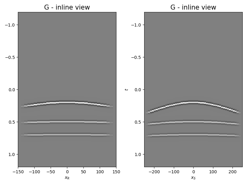
Let’s start by creating a set of hyperbolic events to be used as our MDC kernel
# Input parameters
par = {'ox':-150, 'dx':10, 'nx':31,
       'oy':-250, 'dy':10, 'ny':51,
       'ot':0, 'dt':0.004, 'nt':300,
       'f0': 20, 'nfmax': 200}

t0_m = [0.2]
vrms_m = [700.]
amp_m = [1.]

t0_G = [0.2, 0.5, 0.7]
vrms_G = [800., 1200., 1500.]
amp_G = [1., 0.6, 0.5]

# Taper
tap = taper3d(par['nt'], [par['ny'], par['nx']],
              (5, 5), tapertype='hanning')

# Create axis
t, t2, x, y = makeaxis(par)

# Create wavelet
wav = ricker(t[:41], f0=par['f0'])[0]

# Generate model
m, mwav = hyperbolic2d(x, t, t0_m, vrms_m, amp_m, wav)

# Generate operator
G, Gwav = np.zeros((par['ny'], par['nx'], par['nt'])), \
          np.zeros((par['ny'], par['nx'], par['nt']))
for iy, y0 in enumerate(y):
    G[iy], Gwav[iy] = hyperbolic2d(x-y0, t, t0_G, vrms_G, amp_G, wav)
G, Gwav = G*tap, Gwav*tap

# Add negative part to data and model
m = np.concatenate((np.zeros((par['nx'], par['nt']-1)), m), axis=-1)
mwav = np.concatenate((np.zeros((par['nx'], par['nt']-1)), mwav), axis=-1)
Gwav2 = np.concatenate((np.zeros((par['ny'], par['nx'], par['nt']-1)), Gwav),
                       axis=-1)

# Define MDC linear operator
Gwav_fft = np.fft.rfft(Gwav2, 2*par['nt']-1, axis=-1)
Gwav_fft = Gwav_fft[..., :par['nfmax']]

MDCop = pylops.waveeqprocessing.MDC(Gwav_fft, nt=2 * par['nt']-1, nv=1,
                                    dt=0.004, dr=1., dtype='float32')

# Create data
d = MDCop*m.flatten()
d = d.reshape(par['ny'], 2*par['nt']-1)
Out:
/home/docs/checkouts/readthedocs.org/user_builds/pylops/envs/v1.5.0/lib/python3.6/site-packages/pylops-1.5.0-py3.6.egg/pylops/waveeqprocessing/mdd.py:112: FutureWarning: A new implementation of MDC is provided in v1.5.0. This currently affects only the inner working of the operator, end-users can continue using the operator in the same way. Nevertheless, it is now recommended to start using the operator with transpose=True, as this behaviour will become default in version v2.0.0 and the behaviour with transpose=False will be deprecated.
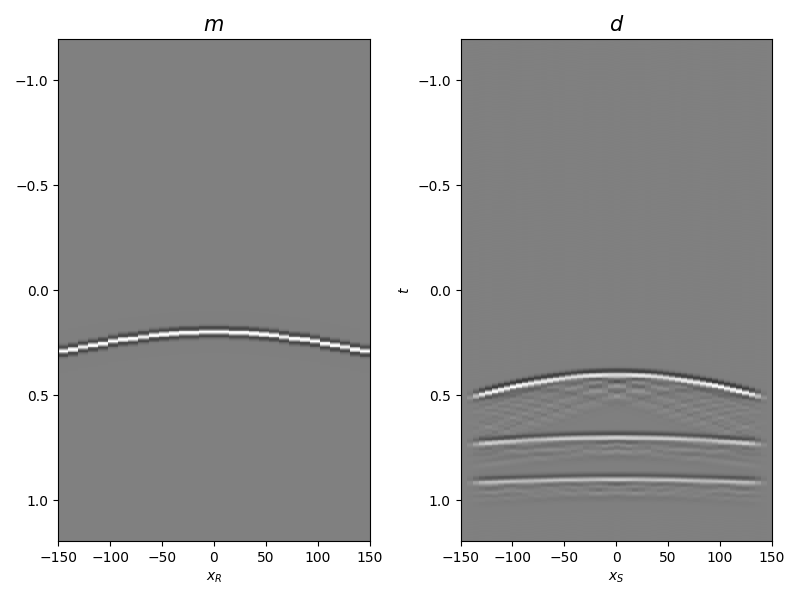
Let’s display what we have so far: operator, input model, and data
fig, axs = plt.subplots(1, 2, figsize=(8, 6))
axs[0].imshow(Gwav2[int(par['ny']/2)].T, aspect='auto',
              interpolation='nearest', cmap='gray',
              vmin=-np.abs(Gwav2.max()), vmax=np.abs(Gwav2.max()),
              extent=(x.min(), x.max(), t2.max(), t2.min()))
axs[0].set_title('G - inline view', fontsize=15)
axs[0].set_xlabel(r'$x_R$')
axs[1].set_ylabel(r'$t$')
axs[1].imshow(Gwav2[:, int(par['nx']/2)].T, aspect='auto',
              interpolation='nearest', cmap='gray',
              vmin=-np.abs(Gwav2.max()), vmax=np.abs(Gwav2.max()),
              extent=(y.min(), y.max(), t2.max(), t2.min()))
axs[1].set_title('G - inline view', fontsize=15)
axs[1].set_xlabel(r'$x_S$')
axs[1].set_ylabel(r'$t$')
fig.tight_layout()

fig, axs = plt.subplots(1, 2, figsize=(8, 6))
axs[0].imshow(mwav.T, aspect='auto', interpolation='nearest', cmap='gray',
              vmin=-np.abs(mwav.max()), vmax=np.abs(mwav.max()),
              extent=(x.min(), x.max(), t2.max(), t2.min()))
axs[0].set_title(r'$m$', fontsize=15)
axs[0].set_xlabel(r'$x_R$')
axs[1].set_ylabel(r'$t$')
axs[1].imshow(d.T, aspect='auto', interpolation='nearest', cmap='gray',
              vmin=-np.abs(d.max()), vmax=np.abs(d.max()),
              extent=(x.min(), x.max(), t2.max(), t2.min()))
axs[1].set_title(r'$d$', fontsize=15)
axs[1].set_xlabel(r'$x_S$')
axs[1].set_ylabel(r'$t$')
fig.tight_layout()
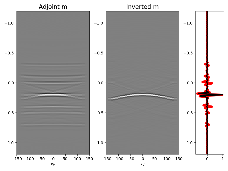
We are now ready to feed our operator to
pylops.waveeqprocessing.MDD and invert back for our input model
minv, madj, psfinv, psfadj = \
pylops.waveeqprocessing.MDD(Gwav, d[:, par['nt'] - 1:],
dt=par['dt'], dr=par['dx'],
nfmax=par['nfmax'], wav=wav,
twosided=True, add_negative=True,
adjoint=True, psf=True,
dtype='complex64', dottest=False,
**dict(damp=1e-4, iter_lim=20, show=0))
fig = plt.figure(figsize=(8, 6))
ax1 = plt.subplot2grid((1, 5), (0, 0), colspan=2)
ax2 = plt.subplot2grid((1, 5), (0, 2), colspan=2)
ax3 = plt.subplot2grid((1, 5), (0, 4))
ax1.imshow(madj.T, aspect='auto', interpolation='nearest', cmap='gray',
vmin=-np.abs(madj.max()), vmax=np.abs(madj.max()),
extent=(x.min(), x.max(), t2.max(), t2.min()))
ax1.set_title('Adjoint m', fontsize=15)
ax1.set_xlabel(r'$x_V$')
axs[1].set_ylabel(r'$t$')
ax2.imshow(minv.T, aspect='auto', interpolation='nearest', cmap='gray',
vmin=-np.abs(minv.max()), vmax=np.abs(minv.max()),
extent=(x.min(), x.max(), t2.max(), t2.min()))
ax2.set_title('Inverted m', fontsize=15)
ax2.set_xlabel(r'$x_V$')
axs[1].set_ylabel(r'$t$')
ax3.plot(madj[int(par['nx']/2)]/np.abs(madj[int(par['nx']/2)]).max(),
t2, 'r', lw=5)
ax3.plot(minv[int(par['nx']/2)]/np.abs(minv[int(par['nx']/2)]).max(),
t2, 'k', lw=3)
ax3.set_ylim([t2[-1], t2[0]])
fig.tight_layout()
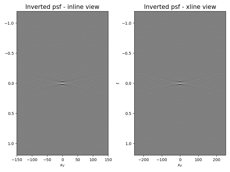
fig, axs = plt.subplots(1, 2, figsize=(8, 6))
axs[0].imshow(psfinv[int(par['nx']/2)].T,
aspect='auto', interpolation='nearest',
vmin=-np.abs(psfinv.max()), vmax=np.abs(psfinv.max()),
cmap='gray', extent=(x.min(), x.max(), t2.max(), t2.min()))
axs[0].set_title('Inverted psf - inline view', fontsize=15)
axs[0].set_xlabel(r'$x_V$')
axs[1].set_ylabel(r'$t$')
axs[1].imshow(psfinv[:, int(par['nx']/2)].T,
aspect='auto', interpolation='nearest',
vmin=-np.abs(psfinv.max()), vmax=np.abs(psfinv.max()),
cmap='gray', extent=(y.min(), y.max(), t2.max(), t2.min()))
axs[1].set_title('Inverted psf - xline view', fontsize=15)
axs[1].set_xlabel(r'$x_V$')
axs[1].set_ylabel(r'$t$')
fig.tight_layout()
We repeat the same procedure but this time we will add a preconditioning
by means of causality_precond parameter, which enforces the inverted
model to be zero in the negative part of the time axis (as expected by
theory). This preconditioning will have the effect of speeding up the
convergence of the iterative solver and thus reduce the computation time
of the deconvolution
minvprec = pylops.waveeqprocessing.MDD(Gwav, d[:, par['nt'] - 1:],
                                       dt=par['dt'], dr=par['dx'],
                                       nfmax=par['nfmax'], wav=wav,
                                       twosided=True, add_negative=True,
                                       adjoint=False, psf=False,
                                       causality_precond=True,
                                       dtype='complex64',
                                       dottest=False,
                                       **dict(damp=1e-4, iter_lim=50, show=0))

# sphinx_gallery_thumbnail_number = 5
fig = plt.figure(figsize=(8, 6))
ax1 = plt.subplot2grid((1, 5), (0, 0), colspan=2)
ax2 = plt.subplot2grid((1, 5), (0, 2), colspan=2)
ax3 = plt.subplot2grid((1, 5), (0, 4))
ax1.imshow(madj.T, aspect='auto', interpolation='nearest', cmap='gray',
           vmin=-np.abs(madj.max()), vmax=np.abs(madj.max()),
           extent=(x.min(), x.max(), t2.max(), t2.min()))
ax1.set_title('Adjoint m', fontsize=15)
ax1.set_xlabel(r'$x_V$')
axs[1].set_ylabel(r'$t$')
ax2.imshow(minvprec.T, aspect='auto', interpolation='nearest', cmap='gray',
           vmin=-np.abs(minvprec.max()), vmax=np.abs(minvprec.max()),
           extent=(x.min(), x.max(), t2.max(), t2.min()))
ax2.set_title('Inverted m', fontsize=15)
ax2.set_xlabel(r'$x_V$')
axs[1].set_ylabel(r'$t$')
ax3.plot(madj[int(par['nx']/2)]/np.abs(madj[int(par['nx']/2)]).max(),
         t2, 'r', lw=5)
ax3.plot(minvprec[int(par['nx']/2)]/np.abs(minv[int(par['nx']/2)]).max(),
         t2, 'k', lw=3)
ax3.set_ylim([t2[-1], t2[0]])
fig.tight_layout()

Total running time of the script: ( 0 minutes 46.921 seconds)