Note
Click here to download the full example code
ISTA and FISTA
This example shows how to use the pylops.optimization.sparsity.ISTA
and pylops.optimization.sparsity.FISTA solvers.
These solvers can be used when the model to retrieve is supposed to have a sparse representation in a certail domain, which mathematically translates to optimizing the following cost function:
import numpy as np
import matplotlib.pyplot as plt

import pylops

plt.close('all')
np.random.seed(0)
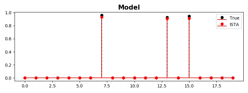
Let’s start with a simple example, where we create a dense mixing matrix and a sparse signal and we use ISTA to recover such a signal. Note that the mixing matrix leads to an underdetermined system of equations (\(N < M\)) so being able to add some extra prior information regarding the sparsity of our desired model is essential to be able to invert such a system.
N, M = 15, 20
Aop = pylops.MatrixMult(np.random.randn(N, M))
x = np.random.rand(M)
x[x < 0.9] = 0
y = Aop*x
# ISTA
eps = 0.5
maxit = 1000
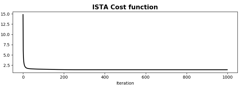
x_ista, niter, cost = pylops.optimization.sparsity.ISTA(Aop, y, maxit, eps=eps,
tol=0, returninfo=True)
fig, ax = plt.subplots(1, 1, figsize=(8, 3))
ax.stem(x, linefmt='k',
markerfmt='ko', label='True')
ax.stem(x_ista, linefmt='--r',
markerfmt='ro', label='ISTA')
ax.set_title('Model', size=15, fontweight='bold')
ax.legend()
plt.tight_layout()
fig, ax = plt.subplots(1, 1, figsize=(8, 3))
ax.plot(cost, 'k', lw=2)
ax.set_title('ISTA Cost function', size=15, fontweight='bold')
ax.set_xlabel('Iteration')
plt.tight_layout()
Out:
/home/docs/checkouts/readthedocs.org/user_builds/pylops/checkouts/v1.6.0/examples/plot_ista.py:47: UserWarning: In Matplotlib 3.3 individual lines on a stem plot will be added as a LineCollection instead of individual lines. This significantly improves the performance of a stem plot. To remove this warning and switch to the new behaviour, set the "use_line_collection" keyword argument to True.
  markerfmt='ko', label='True')
/home/docs/checkouts/readthedocs.org/user_builds/pylops/checkouts/v1.6.0/examples/plot_ista.py:49: UserWarning: In Matplotlib 3.3 individual lines on a stem plot will be added as a LineCollection instead of individual lines. This significantly improves the performance of a stem plot. To remove this warning and switch to the new behaviour, set the "use_line_collection" keyword argument to True.
  markerfmt='ro', label='ISTA')
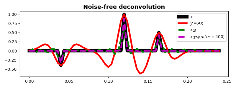
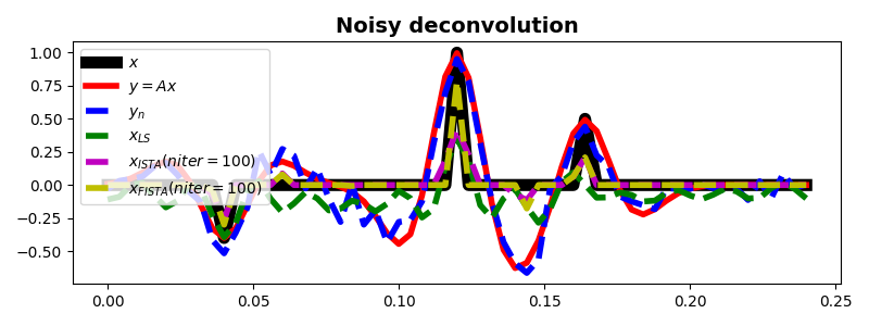
We now consider a more interesting problem problem, wavelet deconvolution
from a signal that we assume being composed by a train of spikes convolved
with a certain wavelet. We will see how solving such a problem with a
least-squares solver such as
pylops.optimization.leastsquares.RegularizedInversion does not
produce the expected results (especially in the presence of noisy data),
conversely using the pylops.optimization.sparsity.ISTA and
pylops.optimization.sparsity.FISTA solvers allows us
to succesfully retrieve the input signal even in the presence of noise.
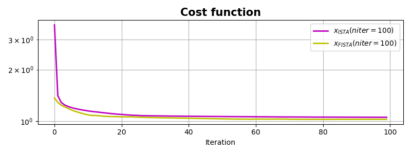
pylops.optimization.sparsity.FISTA shows faster convergence which
is particularly useful for this problem.
nt = 61
dt = 0.004
t = np.arange(nt)*dt
x = np.zeros(nt)
x[10] = -.4
x[int(nt/2)] = 1
x[nt-20] = 0.5

h, th, hcenter = pylops.utils.wavelets.ricker(t[:101], f0=20)

Cop = pylops.signalprocessing.Convolve1D(nt, h=h, offset=hcenter,
                                         dtype='float32')
y = Cop*x
yn = y + np.random.normal(0, 0.1, y.shape)

# noise free
xls = Cop / y

xista, niter, cost = \
    pylops.optimization.sparsity.ISTA(Cop, y, niter=400, eps=5e-1,
                                      tol=1e-8, returninfo=True)

fig, ax = plt.subplots(1, 1, figsize=(8, 3))
ax.plot(t, x, 'k', lw=8, label=r'$x$')
ax.plot(t, y, 'r', lw=4, label=r'$y=Ax$')
ax.plot(t, xls, '--g', lw=4, label=r'$x_{LS}$')
ax.plot(t, xista, '--m', lw=4, label=r'$x_{ISTA} (niter=%d)$' % niter)
ax.set_title('Noise-free deconvolution', fontsize=14, fontweight='bold')
ax.legend()
plt.tight_layout()

# noisy
xls = \
    pylops.optimization.leastsquares.RegularizedInversion(Cop, [], yn,
                                                          returninfo=False,
                                                          **dict(damp=1e-1,
                                                                 atol=1e-3,
                                                                 iter_lim=100,
                                                                 show=0))

xista, niteri, costi = \
    pylops.optimization.sparsity.ISTA(Cop, yn, niter=100, eps=5e-1,
                                      tol=1e-5, returninfo=True)

xfista, niterf, costf = \
    pylops.optimization.sparsity.FISTA(Cop, yn, niter=100, eps=5e-1,
                                       tol=1e-5, returninfo=True)

fig, ax = plt.subplots(1, 1, figsize=(8, 3))
ax.plot(t, x, 'k', lw=8, label=r'$x$')
ax.plot(t, y, 'r', lw=4, label=r'$y=Ax$')
ax.plot(t, yn, '--b', lw=4, label=r'$y_n$')
ax.plot(t, xls, '--g', lw=4, label=r'$x_{LS}$')
ax.plot(t, xista, '--m', lw=4, label=r'$x_{ISTA} (niter=%d)$' % niteri)
ax.plot(t, xfista, '--y', lw=4, label=r'$x_{FISTA} (niter=%d)$' % niterf)
ax.set_title('Noisy deconvolution', fontsize=14, fontweight='bold')
ax.legend()
plt.tight_layout()

fig, ax = plt.subplots(1, 1, figsize=(8, 3))
ax.semilogy(costi, 'm', lw=2, label=r'$x_{ISTA} (niter=%d)$' % niteri)
ax.semilogy(costf, 'y', lw=2, label=r'$x_{FISTA} (niter=%d)$' % niterf)
ax.set_title('Cost function', size=15, fontweight='bold')
ax.set_xlabel('Iteration')
ax.legend()
ax.grid(True, which='both')
plt.tight_layout()
Total running time of the script: ( 0 minutes 1.530 seconds)