Note
Click here to download the full example code
09. Marchenko redatuming by inversion
This example shows how to set-up and run the
pylops.waveeqprocessing.Marchenko inversion using synthetic data.
Let’s start by defining some input parameters and loading the test data
# Input parameters
inputfile = '../testdata/marchenko/input.npz'
vs_zx = [1060, 1200] # virtual source z,x
vel = 2400.0 # velocity
toff = 0.045 # direct arrival time shift
nsmooth = 10 # time window smoothing
nfmax = 1000 # max frequency for MDC (#samples)
niter = 10 # iterations
inputdata = np.load(inputfile)
# Receivers
r = inputdata['r']
nr = r.shape[1]
dr = r[0, 1]-r[0, 0]
# Sources
s = inputdata['s']
ns = s.shape[1]
ds = s[0, 1]-s[0, 0]
# Virtual points
vs = inputdata['vs']
# Density model
rho = inputdata['rho']
z, x = inputdata['z'], inputdata['x']
# Reflection data (R[s, r, t]) and subsurface fields
R = inputdata['R'][:, :, :-100]
R = np.swapaxes(R, 0, 1) # just because of how the data was saved
Gsub = inputdata['Gsub'][:-100]
G0sub = inputdata['G0sub'][:-100]
wav = inputdata['wav']
wav_c = np.argmax(wav)
t = inputdata['t'][:-100]
ot, dt, nt = t[0], t[1]-t[0], len(t)
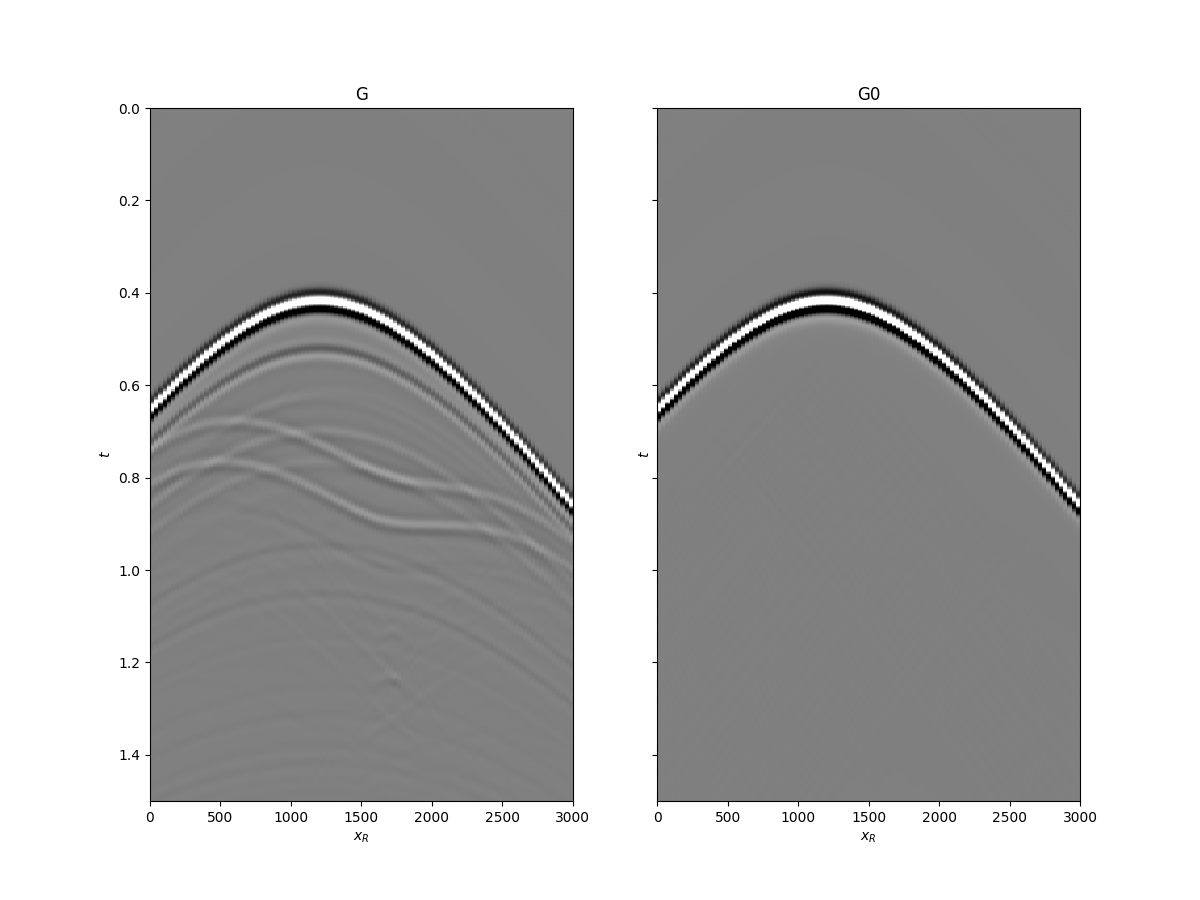
Gsub = np.apply_along_axis(convolve, 0, Gsub, wav, mode='full')
Gsub = Gsub[wav_c:][:nt]
G0sub = np.apply_along_axis(convolve, 0, G0sub, wav, mode='full')
G0sub = G0sub[wav_c:][:nt]
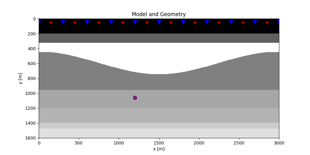
plt.figure(figsize=(10, 5))
plt.imshow(rho, cmap='gray', extent=(x[0], x[-1], z[-1], z[0]))
plt.scatter(s[0, 5::10], s[1, 5::10], marker='*', s=150, c='r', edgecolors='k')
plt.scatter(r[0, ::10], r[1, ::10], marker='v', s=150, c='b', edgecolors='k')
plt.scatter(vs[0], vs[1], marker='.', s=250, c='m', edgecolors='k')
plt.axis('tight')
plt.xlabel('x [m]')
plt.ylabel('y [m]')
plt.title('Model and Geometry')
plt.xlim(x[0], x[-1])
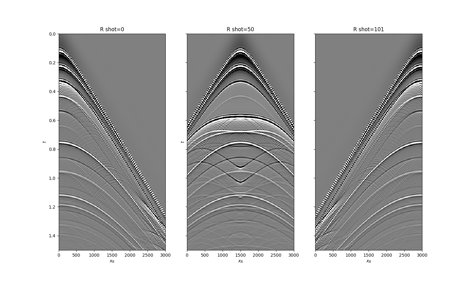
fig, axs = plt.subplots(1, 3, sharey=True, figsize=(15, 9))
axs[0].imshow(R[0].T, cmap='gray', vmin=-1e-2, vmax=1e-2,
extent=(r[0, 0], r[0, -1], t[-1], t[0]))
axs[0].set_title('R shot=0')
axs[0].set_xlabel(r'$x_R$')
axs[0].set_ylabel(r'$t$')
axs[0].axis('tight')
axs[0].set_ylim(1.5, 0)
axs[1].imshow(R[ns//2].T, cmap='gray', vmin=-1e-2, vmax=1e-2,
extent=(r[0, 0], r[0, -1], t[-1], t[0]))
axs[1].set_title('R shot=%d' %(ns//2))
axs[1].set_xlabel(r'$x_R$')
axs[1].set_ylabel(r'$t$')
axs[1].axis('tight')
axs[1].set_ylim(1.5, 0)
axs[2].imshow(R[-1].T, cmap='gray', vmin=-1e-2, vmax=1e-2,
extent=(r[0, 0], r[0, -1], t[-1], t[0]))
axs[2].set_title('R shot=%d' %ns)
axs[2].set_xlabel(r'$x_R$')
axs[2].axis('tight')
axs[2].set_ylim(1.5, 0)
fig, axs = plt.subplots(1, 2, sharey=True, figsize=(12, 9))
axs[0].imshow(Gsub, cmap='gray', vmin=-1e6, vmax=1e6,
extent=(r[0, 0], r[0, -1], t[-1], t[0]))
axs[0].set_title('G')
axs[0].set_xlabel(r'$x_R$')
axs[0].set_ylabel(r'$t$')
axs[0].axis('tight')
axs[0].set_ylim(1.5, 0)
axs[1].imshow(G0sub, cmap='gray', vmin=-1e6, vmax=1e6,
extent=(r[0, 0], r[0, -1], t[-1], t[0]))
axs[1].set_title('G0')
axs[1].set_xlabel(r'$x_R$')
axs[1].set_ylabel(r'$t$')
axs[1].axis('tight')
axs[1].set_ylim(1.5, 0)
Let’s now create an object of the
pylops.waveeqprocessing.Marchenko class and apply redatuming
for a single subsurface point vs.
# direct arrival window
trav = np.sqrt((vs[0]-r[0])**2+(vs[1]-r[1])**2)/vel

MarchenkoWM = Marchenko(R, dt=dt, dr=dr, nfmax=nfmax, wav=wav,
                        toff=toff, nsmooth=nsmooth)

f1_inv_minus, f1_inv_plus, p0_minus, g_inv_minus, g_inv_plus = \
    MarchenkoWM.apply_onepoint(trav, G0=G0sub.T, rtm=True, greens=True,
                               dottest=True, **dict(iter_lim=niter, show=True))
g_inv_tot = g_inv_minus + g_inv_plus
Out:
Dot test passed, v^T(Opu)=491.131956 - u^T(Op^Tv)=491.131956
Dot test passed, v^T(Opu)=464.113195 - u^T(Op^Tv)=464.113195

LSQR            Least-squares solution of  Ax = b
The matrix A has   282598 rows  and   282598 cols
damp = 0.00000000000000e+00   calc_var =        0
atol = 1.00e-08                 conlim = 1.00e+08
btol = 1.00e-08               iter_lim =       10

   Itn      x[0]       r1norm     r2norm   Compatible    LS      Norm A   Cond A
     0  0.00000e+00   3.134e+07  3.134e+07    1.0e+00  3.3e-08
     1  0.00000e+00   1.374e+07  1.374e+07    4.4e-01  9.3e-01   1.1e+00  1.0e+00
     2  0.00000e+00   7.770e+06  7.770e+06    2.5e-01  3.9e-01   1.8e+00  2.2e+00
     3  0.00000e+00   5.750e+06  5.750e+06    1.8e-01  3.3e-01   2.1e+00  3.4e+00
     4  0.00000e+00   3.930e+06  3.930e+06    1.3e-01  3.4e-01   2.5e+00  5.1e+00
     5  0.00000e+00   3.042e+06  3.042e+06    9.7e-02  2.6e-01   2.9e+00  6.8e+00
     6  0.00000e+00   2.423e+06  2.423e+06    7.7e-02  2.2e-01   3.3e+00  8.6e+00
     7  0.00000e+00   1.675e+06  1.675e+06    5.3e-02  2.5e-01   3.6e+00  1.1e+01
     8  0.00000e+00   1.248e+06  1.248e+06    4.0e-02  2.0e-01   3.9e+00  1.3e+01
     9  0.00000e+00   1.004e+06  1.004e+06    3.2e-02  1.5e-01   4.2e+00  1.4e+01
    10  0.00000e+00   7.762e+05  7.762e+05    2.5e-02  1.8e-01   4.4e+00  1.6e+01

LSQR finished
The iteration limit has been reached

istop =       7   r1norm = 7.8e+05   anorm = 4.4e+00   arnorm = 6.1e+05
itn   =      10   r2norm = 7.8e+05   acond = 1.6e+01   xnorm  = 3.6e+07
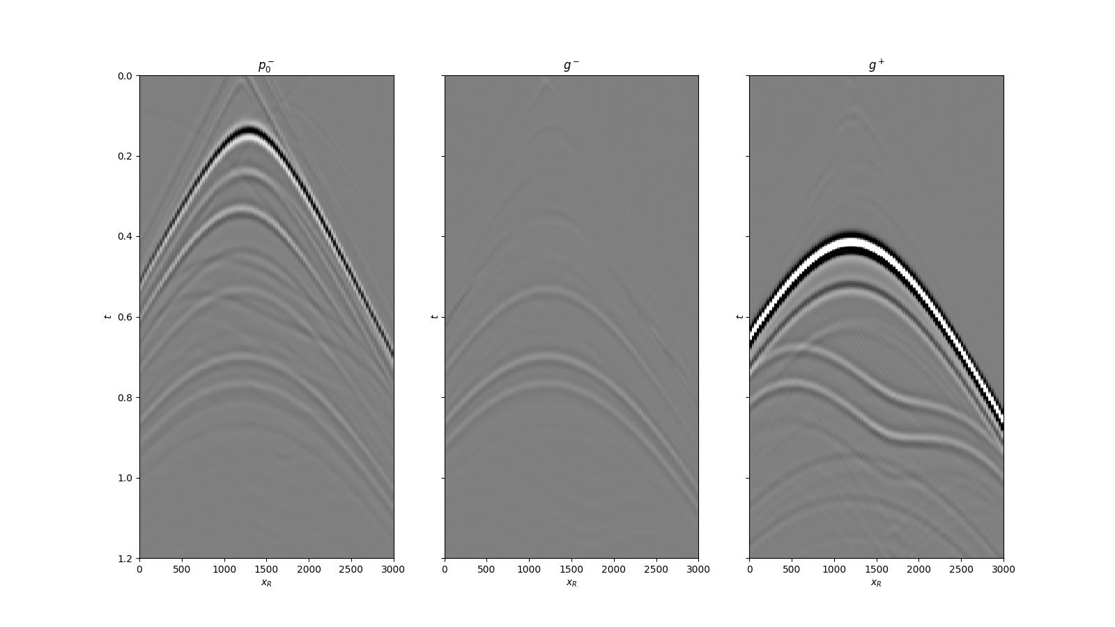
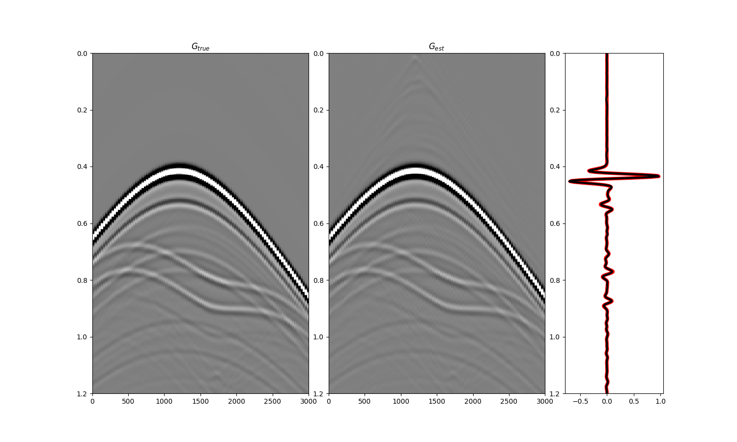
We can now compare the result of Marchenko redatuming via LSQR with standard redatuming
fig, axs = plt.subplots(1, 3, sharey=True, figsize=(16, 9))
axs[0].imshow(p0_minus.T, cmap='gray', vmin=-5e5, vmax=5e5,
              extent=(r[0, 0], r[0, -1], t[-1], -t[-1]))
axs[0].set_title(r'$p_0^-$')
axs[0].set_xlabel(r'$x_R$')
axs[0].set_ylabel(r'$t$')
axs[0].axis('tight')
axs[0].set_ylim(1.2, 0)
axs[1].imshow(g_inv_minus.T, cmap='gray', vmin=-5e5, vmax=5e5,
              extent=(r[0, 0], r[0, -1], t[-1], -t[-1]))
axs[1].set_title(r'$g^-$')
axs[1].set_xlabel(r'$x_R$')
axs[1].set_ylabel(r'$t$')
axs[1].axis('tight')
axs[1].set_ylim(1.2, 0)
axs[2].imshow(g_inv_plus.T, cmap='gray', vmin=-5e5, vmax=5e5,
              extent=(r[0, 0], r[0, -1], t[-1], -t[-1]))
axs[2].set_title(r'$g^+$')
axs[2].set_xlabel(r'$x_R$')
axs[2].set_ylabel(r'$t$')
axs[2].axis('tight')
axs[2].set_ylim(1.2, 0)

fig = plt.figure(figsize=(15, 9))
ax1 = plt.subplot2grid((1, 5), (0, 0), colspan=2)
ax2 = plt.subplot2grid((1, 5), (0, 2), colspan=2)
ax3 = plt.subplot2grid((1, 5), (0, 4))
ax1.imshow(Gsub, cmap='gray', vmin=-5e5, vmax=5e5,
           extent=(r[0, 0], r[0, -1], t[-1], t[0]))
ax1.set_title(r'$G_{true}$')
axs[0].set_xlabel(r'$x_R$')
axs[0].set_ylabel(r'$t$')
ax1.axis('tight')
ax1.set_ylim(1.2, 0)
ax2.imshow(g_inv_tot.T, cmap='gray', vmin=-5e5, vmax=5e5,
           extent=(r[0, 0], r[0, -1], t[-1], -t[-1]))
ax2.set_title(r'$G_{est}$')
axs[1].set_xlabel(r'$x_R$')
axs[1].set_ylabel(r'$t$')
ax2.axis('tight')
ax2.set_ylim(1.2, 0)
ax3.plot(Gsub[:, nr//2]/Gsub.max(), t, 'r', lw=5)
ax3.plot(g_inv_tot[nr//2, nt-1:]/g_inv_tot.max(), t, 'k', lw=3)
ax3.set_ylim(1.2, 0)
Note that Marchenko redatuming can also be applied simultaneously
to multiple subsurface points. Use
pylops.waveeqprocessing.Marchenko.apply_multiplepoints instead of
pylops.waveeqprocessing.Marchenko.apply_onepoint.
Total running time of the script: ( 0 minutes 24.561 seconds)