Note
Click here to download the full example code
Wavelet estimation
This example shows how to use the pylops.avo.prestack.PrestackWaveletModelling to
estimate a wavelet from pre-stack seismic data. This problem can be written in mathematical
form as:
where \(\mathbf{G}\) is an operator that convolves an angle-variant reflectivity series with the wavelet \(\mathbf{w}\) that we aim to retrieve.
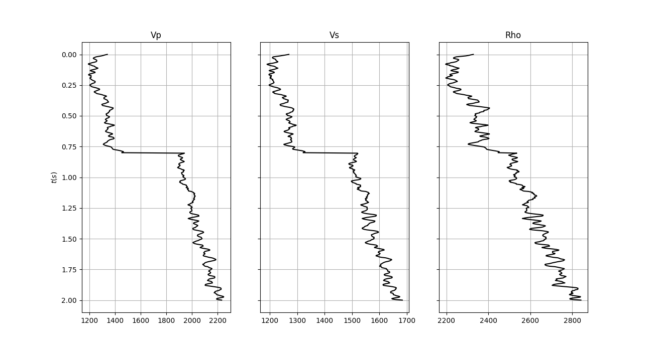
Let’s start by creating the input elastic property profiles and wavelet
nt0 = 501
dt0 = 0.004
ntheta = 21

t0 = np.arange(nt0)*dt0
thetamin, thetamax = 0, 40
theta = np.linspace(thetamin, thetamax, ntheta)

# Elastic property profiles
vp = 1200 + np.arange(nt0) + filtfilt(np.ones(5)/5., 1, np.random.normal(0, 80, nt0))
vs = 600 + vp/2 + filtfilt(np.ones(5)/5., 1, np.random.normal(0, 20, nt0))
rho = 1000 + vp + filtfilt(np.ones(5)/5., 1, np.random.normal(0, 30, nt0))
vp[201:] += 500
vs[201:] += 200
rho[201:] += 100

# Wavelet
ntwav = 41
wavoff = 10
wav, twav, wavc = ricker(t0[:ntwav//2+1], 20)
wav_phase = np.hstack((wav[wavoff:], np.zeros(wavoff)))

# vs/vp profile
vsvp = 0.5
vsvp_z = np.linspace(0.4, 0.6, nt0)

# Model
m = np.stack((np.log(vp), np.log(vs), np.log(rho)), axis=1)

fig, axs = plt.subplots(1, 3, figsize=(13, 7), sharey=True)
axs[0].plot(vp, t0, 'k')
axs[0].set_title('Vp')
axs[0].set_ylabel(r'$t(s)$')
axs[0].invert_yaxis()
axs[0].grid()
axs[1].plot(vs, t0, 'k')
axs[1].set_title('Vs')
axs[1].invert_yaxis()
axs[1].grid()
axs[2].plot(rho, t0, 'k')
axs[2].set_title('Rho')
axs[2].invert_yaxis()
axs[2].grid()
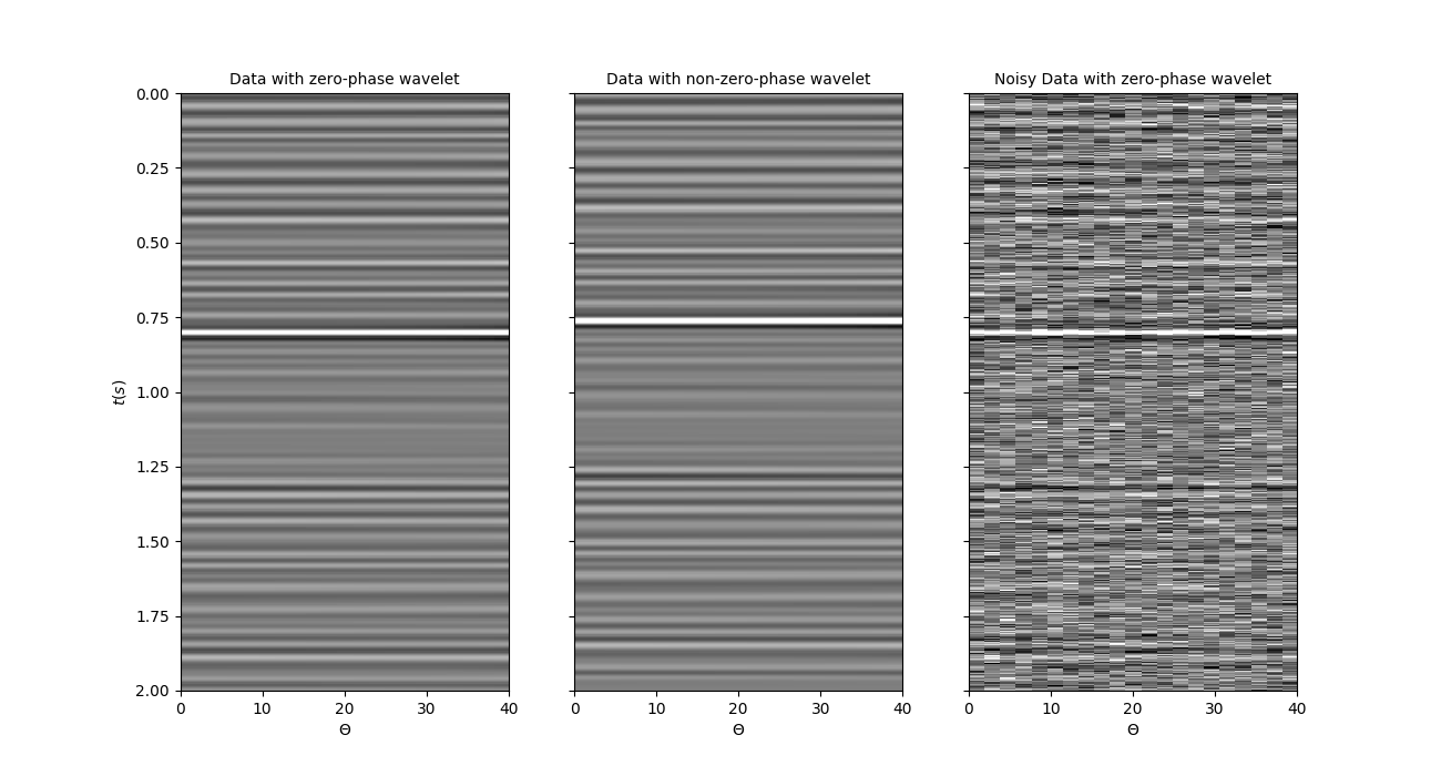
We create now the operators to model a synthetic pre-stack seismic gather with a zero-phase as well as a mixed phase wavelet.
# Create operators
Wavesop = \
    pylops.avo.prestack.PrestackWaveletModelling(m, theta, nwav=ntwav, wavc=wavc,
                                                 vsvp=vsvp, linearization='akirich')
Wavesop_phase = \
    pylops.avo.prestack.PrestackWaveletModelling(m, theta, nwav=ntwav, wavc=wavc,
                                                 vsvp=vsvp, linearization='akirich')
Let’s apply those operators to the elastic model and create some synthetic data
d = (Wavesop*wav).reshape(ntheta, nt0).T
d_phase = (Wavesop_phase*wav_phase).reshape(ntheta, nt0).T

#add noise
dn = d + np.random.normal(0, 3e-2, d.shape)

fig, axs = plt.subplots(1, 3, figsize=(13, 7), sharey=True)
axs[0].imshow(d, cmap='gray', extent=(theta[0], theta[-1], t0[-1], t0[0]),
              vmin=-0.1, vmax=0.1)
axs[0].axis('tight')
axs[0].set_xlabel(r'$\Theta$')
axs[0].set_ylabel(r'$t(s)$')
axs[0].set_title('Data with zero-phase wavelet', fontsize=10)
axs[1].imshow(d_phase, cmap='gray', extent=(theta[0], theta[-1], t0[-1], t0[0]),
              vmin=-0.1, vmax=0.1)
axs[1].axis('tight')
axs[1].set_title('Data with non-zero-phase wavelet', fontsize=10)
axs[1].set_xlabel(r'$\Theta$')
axs[2].imshow(dn, cmap='gray', extent=(theta[0], theta[-1], t0[-1], t0[0]),
              vmin=-0.1, vmax=0.1)
axs[2].axis('tight')
axs[2].set_title('Noisy Data with zero-phase wavelet', fontsize=10)
axs[2].set_xlabel(r'$\Theta$')
Out:
Text(0.5, 0, '$\\Theta$')
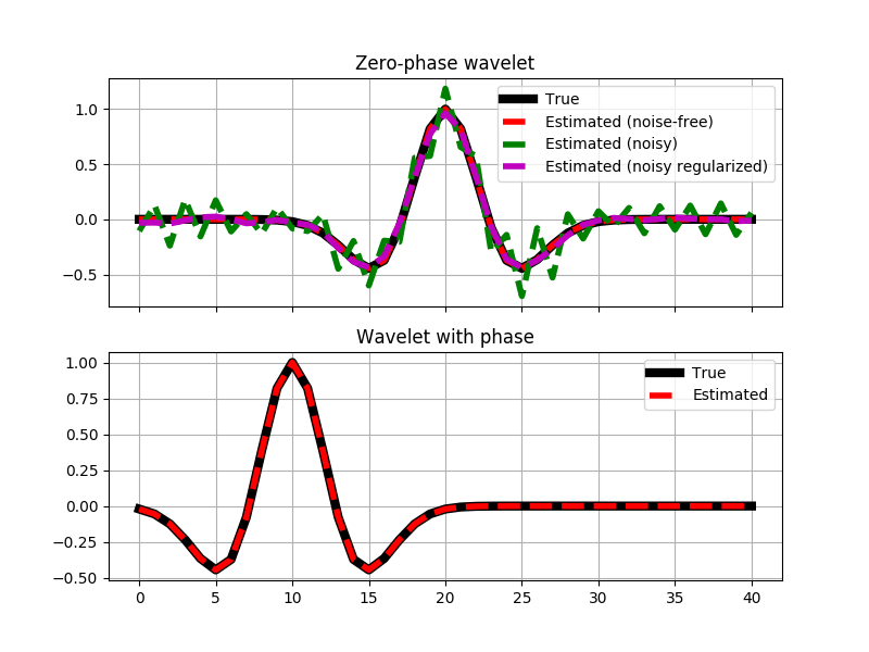
We can invert the data. First we will consider noise-free data, subsequently we will add some noise and add a regularization terms in the inversion process to obtain a well-behaved wavelet also under noise conditions.
wav_est = Wavesop / d.T.flatten()
wav_phase_est = Wavesop_phase / d_phase.T.flatten()
wavn_est = Wavesop / dn.T.flatten()

# Create regularization operator
D2op = pylops.SecondDerivative(ntwav, dtype='float64')

# Invert for wavelet
wavn_reg_est, istop, itn, r1norm, r2norm = \
    pylops.optimization.leastsquares.RegularizedInversion(Wavesop, [D2op], dn.T.flatten(),
                                                          epsRs=[np.sqrt(0.1)], returninfo=True,
                                                          **dict(damp=np.sqrt(1e-4),
                                                                 iter_lim=200, show=0))
As expected, the regularization helps to retrieve a smooth wavelet even under noisy conditions.
# sphinx_gallery_thumbnail_number = 3
fig, axs = plt.subplots(2, 1, sharex=True, figsize=(8, 6))
axs[0].plot(wav, 'k', lw=6, label='True')
axs[0].plot(wav_est, '--r', lw=4, label='Estimated (noise-free)')
axs[0].plot(wavn_est, '--g', lw=4, label='Estimated (noisy)')
axs[0].plot(wavn_reg_est, '--m', lw=4, label='Estimated (noisy regularized)')
axs[0].set_title('Zero-phase wavelet')
axs[0].grid()
axs[0].legend(loc='upper right')
axs[0].axis('tight')
axs[1].plot(wav_phase, 'k', lw=6, label='True')
axs[1].plot(wav_phase_est, '--r', lw=4, label='Estimated')
axs[1].set_title('Wavelet with phase')
axs[1].grid()
axs[1].legend(loc='upper right')
axs[1].axis('tight')
Out:
(-2.0, 42.0, -0.517181248397722, 1.0722467261141773)
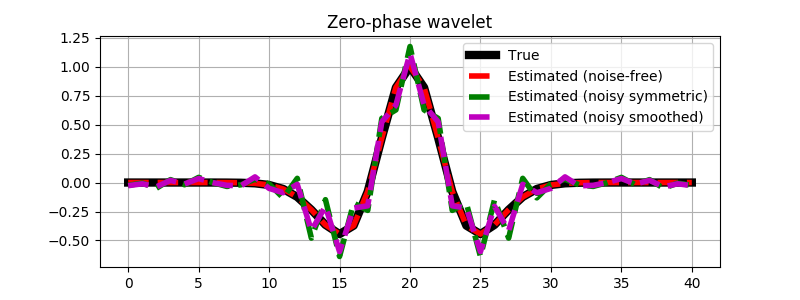
Finally we repeat the same exercise, but this time we use a preconditioner.
Initially, our preconditioner is a pylops.Symmetrize operator
to ensure that our estimated wavelet is zero-phase. After we chain
the pylops.Symmetrize and the pylops.Smoothing1D
operators to also guarantee a smooth wavelet.
# Create symmetrize operator
Sop = pylops.Symmetrize((ntwav+1)//2)

# Create smoothing operator
Smop = pylops.Smoothing1D(5, dims=((ntwav+1)//2,), dtype='float64')

# Invert for wavelet
wavn_prec_est = \
    pylops.optimization.leastsquares.PreconditionedInversion(Wavesop, Sop,
                                                             dn.T.flatten(),
                                                             returninfo=False,
                                                             **dict(damp=np.sqrt(1e-4),
                                                                    iter_lim=200,
                                                                    show=0))

wavn_smooth_est = \
    pylops.optimization.leastsquares.PreconditionedInversion(Wavesop, Sop*Smop,
                                                             dn.T.flatten(),
                                                             returninfo=False,
                                                             **dict(damp=np.sqrt(1e-4),
                                                                    iter_lim=200,
                                                                    show=0))

fig, ax = plt.subplots(1, 1, sharex=True, figsize=(8, 3))
ax.plot(wav, 'k', lw=6, label='True')
ax.plot(wav_est, '--r', lw=4, label='Estimated (noise-free)')
ax.plot(wavn_prec_est, '--g', lw=4, label='Estimated (noisy symmetric)')
ax.plot(wavn_smooth_est, '--m', lw=4, label='Estimated (noisy smoothed)')
ax.set_title('Zero-phase wavelet')
ax.grid()
ax.legend(loc='upper right')
Out:
<matplotlib.legend.Legend object at 0x7f7abb1267b8>
Total running time of the script: ( 0 minutes 4.219 seconds)