Note
Click here to download the full example code
07. Pre-stack (AVO) inversion
Pre-stack inversion represents one step beyond post-stack inversion in that not only the profile of acoustic impedance can be inferred from seismic data, rather a set of elastic parameters is estimated from pre-stack data (i.e., angle gathers) using the information contained in the so-called AVO (amplitude versus offset) response. Such elastic parameters represent vital information for more sophisticated geophysical subsurface characterization than it would be possible to achieve working with post-stack seismic data.
In this tutorial, the pylops.avo.prestack.PrestackLinearModelling
operator is used for modelling of both 1d and 2d synthetic pre-stack seismic
data using 1d profiles or 2d models of different subsurface elastic parameters
(P-wave velocity, S-wave velocity, and density) as input.
where \(\mathbf{m}(t)=[V_P(t), V_S(t), \rho(t)]\) is a vector containing three elastic parameters at time \(t\), \(G_i(t, \theta)\) are the coefficients of the AVO parametrization used to model pre-stack data and \(w(t)\) is the time domain seismic wavelet. In compact form:
where \(\mathbf{W}\) is a convolution operator, \(\mathbf{G}\) is
the AVO modelling operator, \(\mathbf{D}\) is a block-diagonal
derivative operator, and \(\mathbf{m}\) is the input model.
Subsequently the elastic parameters are estimated via the
pylops.avo.prestack.PrestackInversion module.
Once again, a two-steps inversion strategy can also be used to deal
with the case of noisy data.
Let’s start with a 1d example. A synthetic profile of acoustic impedance
is created and data is modelled using both the dense and linear operator
version of pylops.avo.prestack.PrestackLinearModelling operator
# sphinx_gallery_thumbnail_number = 5

# model
nt0 = 301
dt0 = 0.004

t0 = np.arange(nt0)*dt0
vp = 1200 + np.arange(nt0) + \
     filtfilt(np.ones(5)/5., 1, np.random.normal(0, 80, nt0))
vs = 600  + vp/2 + \
     filtfilt(np.ones(5)/5., 1, np.random.normal(0, 20, nt0))
rho = 1000 + vp + \
      filtfilt(np.ones(5)/5., 1, np.random.normal(0, 30, nt0))
vp[131:] += 500
vs[131:] += 200
rho[131:] += 100
vsvp = 0.5
m = np.stack((np.log(vp), np.log(vs), np.log(rho)), axis=1)

# background model
nsmooth = 50
mback = filtfilt(np.ones(nsmooth)/float(nsmooth), 1, m, axis=0)

# angles
ntheta = 21
thetamin, thetamax = 0, 40
theta = np.linspace(thetamin, thetamax, ntheta)

# wavelet
ntwav = 41
wav = ricker(t0[:ntwav//2+1], 15)[0]

# lop
PPop = \
    pylops.avo.prestack.PrestackLinearModelling(wav, theta,
                                                vsvp=vsvp, nt0=nt0,
                                                linearization='akirich')

# dense
PPop_dense = \
    pylops.avo.prestack.PrestackLinearModelling(wav, theta,
                                                vsvp=vsvp, nt0=nt0,
                                                linearization='akirich',
                                                explicit=True)

# data lop
dPP = PPop*m.flatten()
dPP = dPP.reshape(nt0, ntheta)

# data dense
dPP_dense = PPop_dense*m.T.flatten()
dPP_dense = dPP_dense.reshape(ntheta, nt0).T

# noisy data
dPPn_dense = dPP_dense + np.random.normal(0, 1e-2, dPP_dense.shape)
We can now invert our data and retreive elastic profiles for both noise-free
and noisy data using pylops.avo.prestack.PrestackInversion.
# dense
minv_dense, dPP_dense_res = \
    pylops.avo.prestack.PrestackInversion(dPP_dense, theta, wav, m0=mback,
                                          linearization='akirich',
                                          explicit=True, returnres=True,
                                          **dict(cond=1e-10))

# lop
minv, dPP_res = \
    pylops.avo.prestack.PrestackInversion(dPP, theta, wav, m0=mback,
                                          linearization='akirich',
                                          explicit=False, returnres=True,
                                          **dict(damp=1e-10, iter_lim=2000))

# dense noisy
minv_dense_noise, dPPn_dense_res = \
    pylops.avo.prestack.PrestackInversion(dPPn_dense, theta, wav, m0=mback,
                                          linearization='akirich',
                                          explicit=True,
                                          returnres=True, **dict(cond=1e-1))

# lop noisy (with vertical smoothing)
minv_noise, dPPn_res = \
    pylops.avo.prestack.PrestackInversion(dPPn_dense, theta, wav, m0=mback,
                                          linearization='akirich',
                                          explicit=False,
                                          epsR=5e-1, returnres=True,
                                          **dict(damp=1e-1, iter_lim=100))
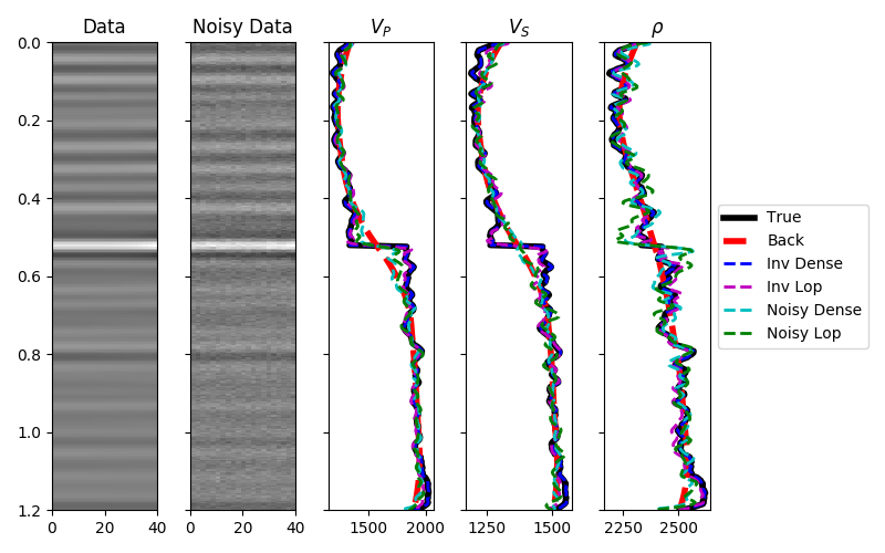
The data, inverted models and residuals are now displayed.
# Data and model
fig, (axd, axdn, axvp, axvs, axrho) = \
plt.subplots(1, 5, figsize=(8, 5), sharey=True)
axd.imshow(dPP_dense, cmap='gray',
extent=(theta[0], theta[-1], t0[-1], t0[0]),
vmin=-np.abs(dPP_dense).max(), vmax=np.abs(dPP_dense).max())
axd.set_title('Data')
axd.axis('tight')
axdn.imshow(dPPn_dense, cmap='gray',
extent=(theta[0], theta[-1], t0[-1], t0[0]),
vmin=-np.abs(dPP_dense).max(), vmax=np.abs(dPP_dense).max())
axdn.set_title('Noisy Data')
axdn.axis('tight')
axvp.plot(vp, t0, 'k', lw=4, label='True')
axvp.plot(np.exp(mback[:, 0]), t0, '--r', lw=4, label='Back')
axvp.plot(np.exp(minv_dense[:, 0]), t0, '--b', lw=2, label='Inv Dense')
axvp.plot(np.exp(minv[:, 0]), t0, '--m', lw=2, label='Inv Lop')
axvp.plot(np.exp(minv_dense_noise[:, 0]), t0, '--c', lw=2, label='Noisy Dense')
axvp.plot(np.exp(minv_noise[:, 0]), t0, '--g', lw=2, label='Noisy Lop')
axvp.set_title(r'$V_P$')
axvs.plot(vs, t0, 'k', lw=4, label='True')
axvs.plot(np.exp(mback[:, 1]), t0, '--r', lw=4, label='Back')
axvs.plot(np.exp(minv_dense[:, 1]), t0, '--b', lw=2, label='Inv Dense')
axvs.plot(np.exp(minv[:, 1]), t0, '--m', lw=2, label='Inv Lop')
axvs.plot(np.exp(minv_dense_noise[:, 1]), t0, '--c', lw=2, label='Noisy Dense')
axvs.plot(np.exp(minv_noise[:, 1]), t0, '--g', lw=2, label='Noisy Lop')
axvs.set_title(r'$V_S$')
axrho.plot(rho, t0, 'k', lw=4, label='True')
axrho.plot(np.exp(mback[:, 2]), t0, '--r', lw=4, label='Back')
axrho.plot(np.exp(minv_dense[:, 2]), t0, '--b', lw=2, label='Inv Dense')
axrho.plot(np.exp(minv[:, 2]), t0, '--m', lw=2, label='Inv Lop')
axrho.plot(np.exp(minv_dense_noise[:, 2]),
t0, '--c', lw=2, label='Noisy Dense')
axrho.plot(np.exp(minv_noise[:, 2]), t0, '--g', lw=2, label='Noisy Lop')
axrho.set_title(r'$\rho$')
axrho.legend(loc='center left', bbox_to_anchor=(1, 0.5))
axd.axis('tight')
plt.tight_layout()
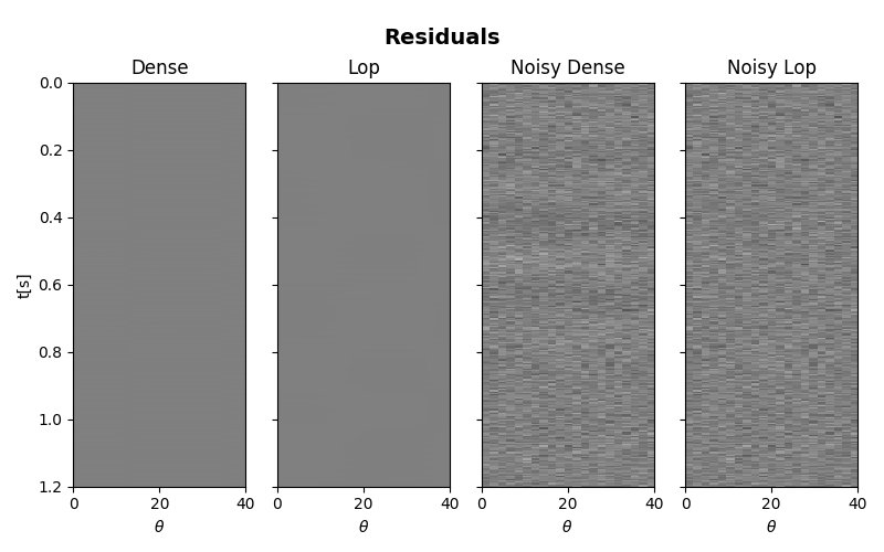
# Residuals
fig, axs = plt.subplots(1, 4, figsize=(8, 5), sharey=True)
fig.suptitle('Residuals', fontsize=14,
fontweight='bold', y=0.95)
im = axs[0].imshow(dPP_dense_res, cmap='gray',
extent=(theta[0], theta[-1], t0[-1], t0[0]),
vmin=-0.1, vmax=0.1)
axs[0].set_title('Dense')
axs[0].set_xlabel(r'$\theta$')
axs[0].set_ylabel('t[s]')
axs[0].axis('tight')
axs[1].imshow(dPP_res, cmap='gray',
extent=(theta[0], theta[-1], t0[-1], t0[0]),
vmin=-0.1, vmax=0.1)
axs[1].set_title('Lop')
axs[1].set_xlabel(r'$\theta$')
axs[1].axis('tight')
axs[2].imshow(dPPn_dense_res, cmap='gray',
extent=(theta[0], theta[-1], t0[-1], t0[0]),
vmin=-0.1, vmax=0.1)
axs[2].set_title('Noisy Dense')
axs[2].set_xlabel(r'$\theta$')
axs[2].axis('tight')
axs[3].imshow(dPPn_res, cmap='gray',
extent=(theta[0], theta[-1], t0[-1], t0[0]),
vmin=-0.1, vmax=0.1)
axs[3].set_title('Noisy Lop')
axs[3].set_xlabel(r'$\theta$')
axs[3].axis('tight')
plt.tight_layout()
plt.subplots_adjust(top=0.85)
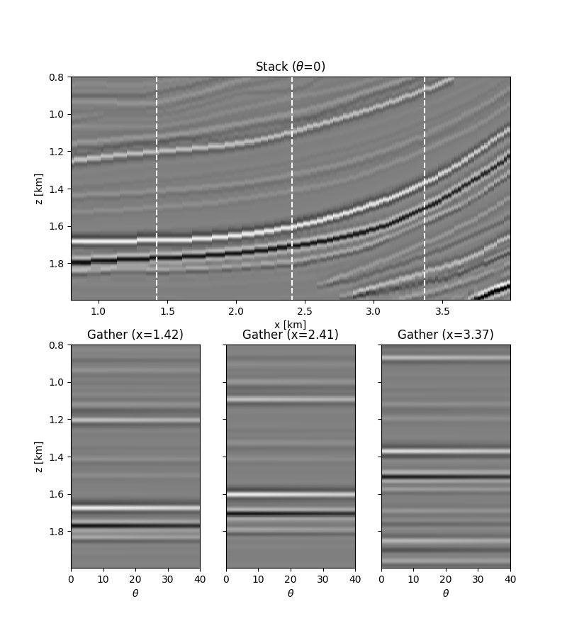
We move now to a 2d example. First of all the model is loaded and data generated.
# model
inputfile = '../testdata/avo/poststack_model.npz'

model = np.load(inputfile)
x, z = model['x'][::6]/1000., model['z'][:300]/1000.
nx, nz = len(x), len(z)
m = 1000*model['model'][:300, ::6]

mvp = m.copy()
mvs = m/2
mrho = m/3+300
m = np.log(np.stack((mvp, mvs, mrho), axis=1))

# smooth model
nsmoothz, nsmoothx = 30, 25
mback = filtfilt(np.ones(nsmoothz)/float(nsmoothz), 1, m, axis=0)
mback = filtfilt(np.ones(nsmoothx)/float(nsmoothx), 1, mback, axis=2)

# dense operator
PPop_dense = \
    pylops.avo.prestack.PrestackLinearModelling(wav, theta, vsvp=vsvp,
                                                nt0=nz, spatdims=(nx,),
                                                linearization='akirich',
                                                explicit=True)

# lop operator
PPop = pylops.avo.prestack.PrestackLinearModelling(wav, theta, vsvp=vsvp,
                                                   nt0=nz, spatdims=(nx,),
                                                   linearization='akirich')

# data
dPP = PPop_dense*m.swapaxes(0, 1).flatten()
dPP = dPP.reshape(ntheta, nz, nx).swapaxes(0, 1)
dPPn = dPP + np.random.normal(0, 5e-2, dPP.shape)
Finally we perform the same 4 different inversions as in the post-stack tutorial (see 06. Post-stack inversion for more details).
# dense inversion with noise-free data
minv_dense = \
    pylops.avo.prestack.PrestackInversion(dPP, theta, wav, m0=mback,
                                          explicit=True,
                                          simultaneous=False)

# dense inversion with noisy data
minv_dense_noisy = \
    pylops.avo.prestack.PrestackInversion(dPPn, theta, wav, m0=mback,
                                          explicit=True, epsI=4e-2,
                                          simultaneous=False)

# spatially regularized lop inversion with noisy data
minv_lop_reg = \
    pylops.avo.prestack.PrestackInversion(dPPn, theta, wav,
                                          m0=minv_dense_noisy,
                                          explicit=False, epsR=1e1,
                                          **dict(damp=np.sqrt(1e-4),
                                                 iter_lim=20))

# blockiness promoting inversion with noisy data
minv_blocky = \
    pylops.avo.prestack.PrestackInversion(dPPn, theta, wav,
                                          m0=mback,
                                          explicit=False,
                                          epsR=0.4, epsRL1=0.1,
                                          **dict(mu=0.1,
                                                 niter_outer=3,
                                                 niter_inner=3,
                                                 iter_lim=5, damp=1e-3))
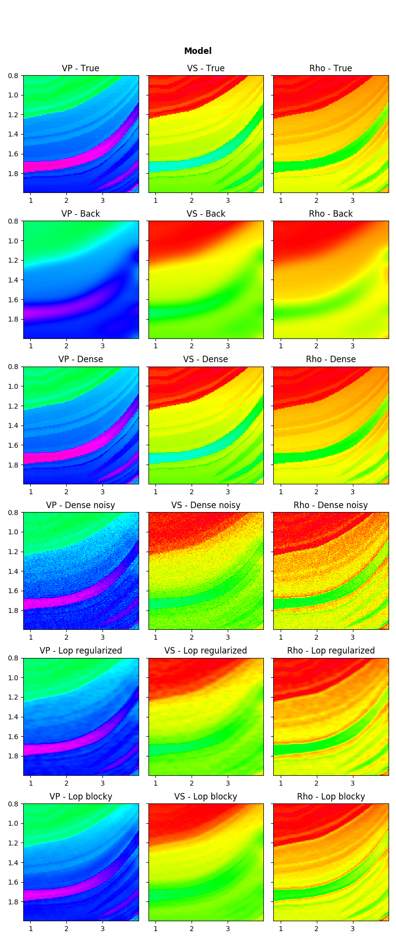
Let’s now visualize the inverted elastic parameters for the different scenarios
def plotmodel(axs, m, x, z, vmin, vmax,
params=('VP', 'VS', 'Rho'),
cmap='gist_rainbow', title=None):
"""Quick visualization of model
"""
for ip, param in enumerate(params):
axs[ip].imshow(m[:, ip],
extent=(x[0], x[-1], z[-1], z[0]),
vmin=vmin, vmax=vmax, cmap=cmap)
axs[ip].set_title('%s - %s' %(param, title))
axs[ip].axis('tight')
plt.setp(axs[1].get_yticklabels(), visible=False)
plt.setp(axs[2].get_yticklabels(), visible=False)
# data
fig = plt.figure(figsize=(8, 9))
ax1 = plt.subplot2grid((2, 3), (0, 0), colspan=3)
ax2 = plt.subplot2grid((2, 3), (1, 0))
ax3 = plt.subplot2grid((2, 3), (1, 1), sharey=ax2)
ax4 = plt.subplot2grid((2, 3), (1, 2), sharey=ax2)
ax1.imshow(dPP[:, 0], cmap='gray',
extent=(x[0], x[-1], z[-1], z[0]),
vmin=-0.4, vmax=0.4)
ax1.vlines([x[nx//5], x[nx//2], x[4*nx//5]], ymin=z[0], ymax=z[-1],
colors='w', linestyles='--')
ax1.set_xlabel('x [km]')
ax1.set_ylabel('z [km]')
ax1.set_title(r'Stack ($\theta$=0)')
ax1.axis('tight')
ax2.imshow(dPP[:, :, nx//5], cmap='gray',
extent=(theta[0], theta[-1], z[-1], z[0]),
vmin=-0.4, vmax=0.4)
ax2.set_xlabel(r'$\theta$')
ax2.set_ylabel('z [km]')
ax2.set_title(r'Gather (x=%.2f)' % x[nx//5])
ax2.axis('tight')
ax3.imshow(dPP[:, :, nx//2], cmap='gray',
extent=(theta[0], theta[-1], z[-1], z[0]),
vmin=-0.4, vmax=0.4)
ax3.set_xlabel(r'$\theta$')
ax3.set_title(r'Gather (x=%.2f)' % x[nx//2])
ax3.axis('tight')
ax4.imshow(dPP[:, :, 4*nx//5], cmap='gray',
extent=(theta[0], theta[-1], z[-1], z[0]),
vmin=-0.4, vmax=0.4)
ax4.set_xlabel(r'$\theta$')
ax4.set_title(r'Gather (x=%.2f)' % x[4*nx//5])
ax4.axis('tight')
plt.setp(ax3.get_yticklabels(), visible=False)
plt.setp(ax4.get_yticklabels(), visible=False)
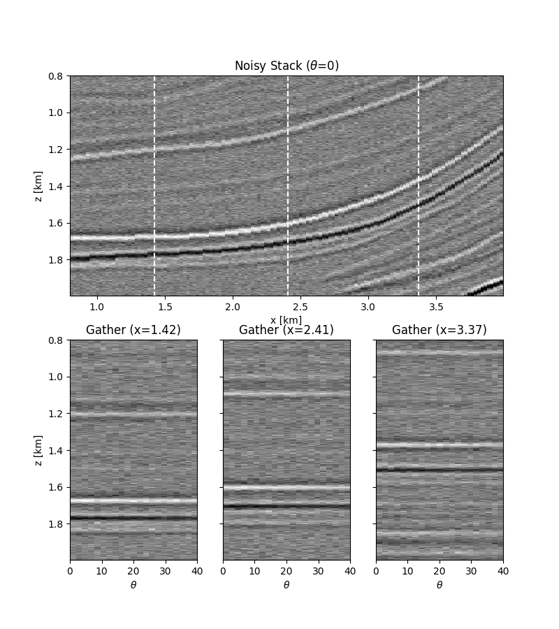
# noisy data
fig = plt.figure(figsize=(8, 9))
ax1 = plt.subplot2grid((2, 3), (0, 0), colspan=3)
ax2 = plt.subplot2grid((2, 3), (1, 0))
ax3 = plt.subplot2grid((2, 3), (1, 1), sharey=ax2)
ax4 = plt.subplot2grid((2, 3), (1, 2), sharey=ax2)
ax1.imshow(dPPn[:, 0], cmap='gray',
extent=(x[0], x[-1], z[-1], z[0]),
vmin=-0.4, vmax=0.4)
ax1.vlines([x[nx//5], x[nx//2], x[4*nx//5]], ymin=z[0], ymax=z[-1],
colors='w', linestyles='--')
ax1.set_xlabel('x [km]')
ax1.set_ylabel('z [km]')
ax1.set_title(r'Noisy Stack ($\theta$=0)')
ax1.axis('tight')
ax2.imshow(dPPn[:, :, nx//5], cmap='gray',
extent=(theta[0], theta[-1], z[-1], z[0]),
vmin=-0.4, vmax=0.4)
ax2.set_xlabel(r'$\theta$')
ax2.set_ylabel('z [km]')
ax2.set_title(r'Gather (x=%.2f)' % x[nx//5])
ax2.axis('tight')
ax3.imshow(dPPn[:, :, nx//2], cmap='gray',
extent=(theta[0], theta[-1], z[-1], z[0]),
vmin=-0.4, vmax=0.4)
ax3.set_title(r'Gather (x=%.2f)' % x[nx//2])
ax3.set_xlabel(r'$\theta$')
ax3.axis('tight')
ax4.imshow(dPPn[:, :, 4*nx//5], cmap='gray',
extent=(theta[0], theta[-1], z[-1], z[0]),
vmin=-0.4, vmax=0.4)
ax4.set_xlabel(r'$\theta$')
ax4.set_title(r'Gather (x=%.2f)' % x[4*nx//5])
ax4.axis('tight')
plt.setp(ax3.get_yticklabels(), visible=False)
plt.setp(ax4.get_yticklabels(), visible=False)
# inverted models
fig, axs = plt.subplots(6, 3, figsize=(8, 19))
fig.suptitle('Model', fontsize=12, fontweight='bold', y=0.95)
plotmodel(axs[0], m, x, z, m.min(),
m.max(), title='True')
plotmodel(axs[1], mback, x, z, m.min(),
m.max(), title='Back')
plotmodel(axs[2], minv_dense, x, z,
m.min(), m.max(), title='Dense')
plotmodel(axs[3], minv_dense_noisy, x, z,
m.min(), m.max(), title='Dense noisy')
plotmodel(axs[4], minv_lop_reg, x, z,
m.min(), m.max(), title='Lop regularized')
plotmodel(axs[5], minv_blocky, x, z,
m.min(), m.max(), title='Lop blocky')
plt.tight_layout()
plt.subplots_adjust(top=0.92)
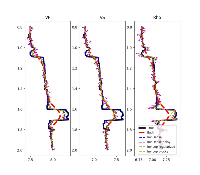
fig, axs = plt.subplots(1, 3, figsize=(8, 7))
for ip, param in enumerate(['VP', 'VS', 'Rho']):
axs[ip].plot(m[:, ip, nx//2], z, 'k', lw=4, label='True')
axs[ip].plot(mback[:, ip, nx//2], z, '--r', lw=4, label='Back')
axs[ip].plot(minv_dense[:, ip, nx//2], z, '--b', lw=2, label='Inv Dense')
axs[ip].plot(minv_dense_noisy[:, ip, nx//2], z, '--m', lw=2,
label='Inv Dense noisy')
axs[ip].plot(minv_lop_reg[:, ip, nx//2], z, '--g', lw=2,
label='Inv Lop regularized')
axs[ip].plot(minv_blocky[:, ip, nx // 2], z, '--y', lw=2,
label='Inv Lop blocky')
axs[ip].set_title(param)
axs[ip].invert_yaxis()
axs[2].legend(loc=8, fontsize='small')
Out:
<matplotlib.legend.Legend object at 0x7f7ab952aac8>
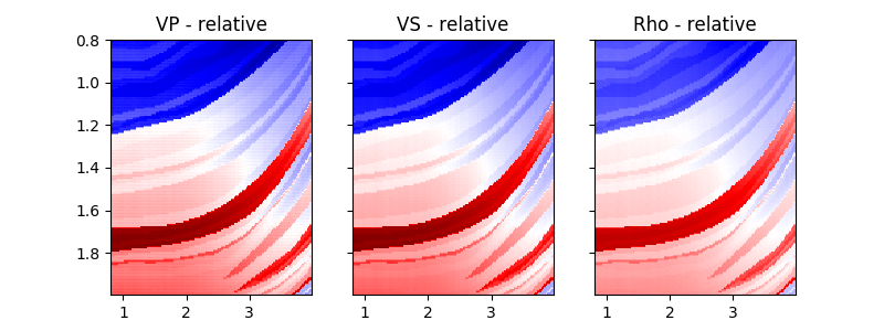
While the background model m0 has been provided in all the examples so
far, it is worth showing that the module
pylops.avo.prestack.PrestackInversion can also produce so-called
relative elastic parameters (i.e., variations from an average medium
property) when the background model m0 is not available.
dminv = \
pylops.avo.prestack.PrestackInversion(dPP, theta, wav, m0=None,
explicit=True,
simultaneous=False)
fig, axs = plt.subplots(1, 3, figsize=(8, 3))
plotmodel(axs, dminv, x, z, -dminv.max(), dminv.max(),
cmap='seismic', title='relative')
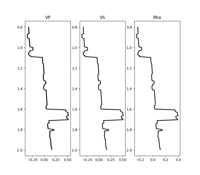
fig, axs = plt.subplots(1, 3, figsize=(8, 7))
for ip, param in enumerate(['VP', 'VS', 'Rho']):
axs[ip].plot(dminv[:, ip, nx//2], z, 'k', lw=2)
axs[ip].set_title(param)
axs[ip].invert_yaxis()
Total running time of the script: ( 0 minutes 39.272 seconds)