Note
Click here to download the full example code
Pre-stack modelling
This example shows how to create pre-stack angle gathers using
the pylops.avo.prestack.PrestackLinearModelling operator.
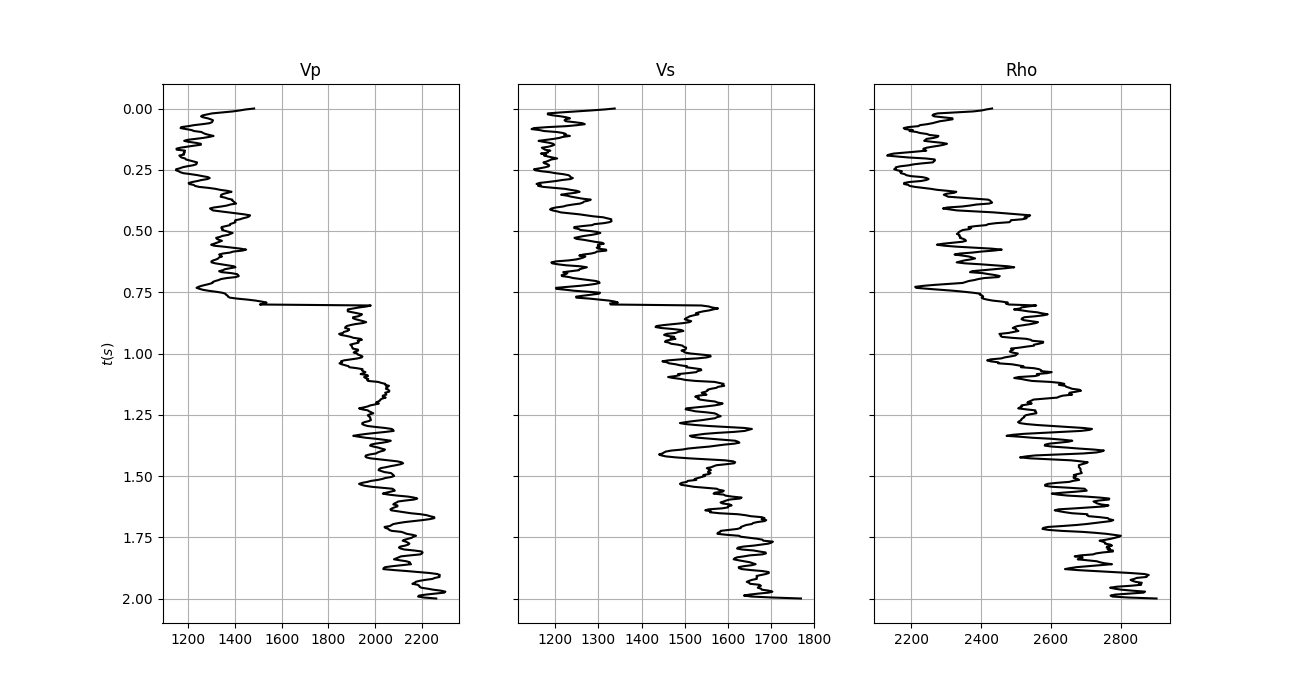
Let’s start by creating the input elastic property profiles and wavelet
nt0 = 501
dt0 = 0.004
ntheta = 21

t0 = np.arange(nt0)*dt0
thetamin, thetamax = 0, 40
theta = np.linspace(thetamin, thetamax, ntheta)

# Elastic property profiles
vp = 1200 + np.arange(nt0) + filtfilt(np.ones(5)/5., 1,
                                      np.random.normal(0, 160, nt0))
vs = 600 + vp/2 + filtfilt(np.ones(5)/5., 1, np.random.normal(0, 100, nt0))
rho = 1000 + vp + filtfilt(np.ones(5)/5., 1, np.random.normal(0, 120, nt0))
vp[201:] += 500
vs[201:] += 200
rho[201:] += 100

# Wavelet
ntwav = 81
wav, twav, wavc = ricker(t0[:ntwav//2+1], 5)

# vs/vp profile
vsvp = 0.5
vsvp_z = np.linspace(0.4, 0.6, nt0)

# Model
m = np.stack((np.log(vp), np.log(vs), np.log(rho)), axis=1)

fig, axs = plt.subplots(1, 3, figsize=(13, 7), sharey=True)
axs[0].plot(vp, t0, 'k')
axs[0].set_title('Vp')
axs[0].set_ylabel(r'$t(s)$')
axs[0].invert_yaxis()
axs[0].grid()
axs[1].plot(vs, t0, 'k')
axs[1].set_title('Vs')
axs[1].invert_yaxis()
axs[1].grid()
axs[2].plot(rho, t0, 'k')
axs[2].set_title('Rho')
axs[2].invert_yaxis()
axs[2].grid()
We create now the operators to model a synthetic pre-stack seismic gather
with a zero-phase using both a constant and a depth-variant vsvp profile
# constant vsvp
PPop_const = \
    pylops.avo.prestack.PrestackLinearModelling(wav, theta, vsvp=vsvp, nt0=nt0,
                                                linearization='akirich')

# depth-variant vsvp
PPop_variant = \
    pylops.avo.prestack.PrestackLinearModelling(wav, theta, vsvp=vsvp_z,
                                                linearization='akirich')
Let’s apply those operators to the elastic model and create some synthetic data
dPP_const = PPop_const *m.flatten()
dPP_const = dPP_const.reshape(nt0, ntheta)

dPP_variant = PPop_variant *m.flatten()
dPP_variant = dPP_variant.reshape(nt0, ntheta)
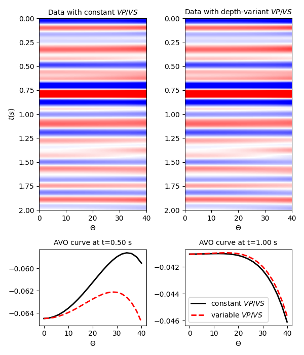
Finally we visualize the two datasets
# sphinx_gallery_thumbnail_number = 2
fig = plt.figure(figsize=(6, 7))
ax1 = plt.subplot2grid((3, 2), (0, 0), rowspan=2)
ax2 = plt.subplot2grid((3, 2), (0, 1), rowspan=2)
ax3 = plt.subplot2grid((3, 2), (2, 0))
ax4 = plt.subplot2grid((3, 2), (2, 1))
ax1.imshow(dPP_const, cmap='bwr',
           extent=(theta[0], theta[-1], t0[-1], t0[0]),
           vmin=-0.1, vmax=0.1)
ax1.set_xlabel(r'$\Theta$')
ax1.set_ylabel(r'$t(s)$')
ax1.set_title(r'Data with constant $VP/VS$', fontsize=10)
ax1.axis('tight')
ax2.imshow(dPP_variant, cmap='bwr',
           extent=(theta[0], theta[-1], t0[-1], t0[0]),
           vmin=-0.1, vmax=0.1)
ax2.set_title(r'Data with depth-variant $VP/VS$', fontsize=10)
ax2.set_xlabel(r'$\Theta$')
ax2.axis('tight')
ax3.plot(theta, dPP_const[nt0//4], 'k', lw=2)
ax3.plot(theta, dPP_variant[nt0//4], '--r', lw=2)
ax3.set_title('AVO curve at t=%.2f s' % t0[nt0//4], fontsize=10)
ax3.set_xlabel(r'$\Theta$')
ax4.plot(theta, dPP_const[nt0//2], 'k', lw=2, label=r'constant $VP/VS$')
ax4.plot(theta, dPP_variant[nt0//2], '--r', lw=2, label=r'variable $VP/VS$')
ax4.set_title('AVO curve at t=%.2f s' % t0[nt0//2], fontsize=10)
ax4.set_xlabel(r'$\Theta$')
ax4.legend()
plt.tight_layout()
Total running time of the script: ( 0 minutes 0.702 seconds)