Seislet transform

This example shows how to use the pylops.signalprocessing.Seislet operator. This operator the forward, adjoint and inverse Seislet transform that is a modification of the well-know Wavelet transform where local slopes are used in the prediction and update steps to further improve the prediction of a trace from its previous (or subsequent) one and reduce the amount of information passed to the subsequent scale. While this transform was initially developed in the context of processing and compression of seismic data, it is also suitable to any other oscillatory dataset such as GPR or Acoustic recordings.

import numpy as np
import matplotlib.pyplot as plt

import pylops

plt.close('all')

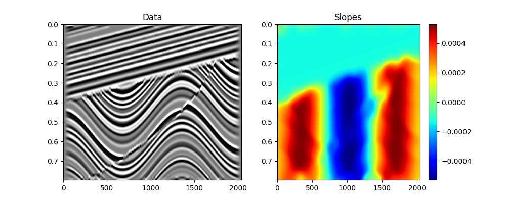
In this example we use the same benchmark dataset that was used in the original paper describing the Seislet transform. First, local slopes are estimated using pylops.utils.signalprocessing.slope_estimate.

inputfile='../testdata/sigmoid.npz'

d = np.load(inputfile)
d = d['sigmoid']
nx, nt = d.shape
dx, dt = 8, 0.004
x, t = np.arange(nx) * dx, np.arange(nt) * dt

# slope estimation
slope = -pylops.utils.signalprocessing.slope_estimate(d.T, dt, dx, smooth=6)[0]

clip = 0.002
fig, axs = plt.subplots(1, 2, figsize=(10, 4))
axs[0].imshow(d.T, cmap='gray', vmin=-clip, vmax=clip,
              extent = (x[0], x[-1], t[-1], t[0]))
axs[0].set_title('Data')
axs[0].axis('tight')
im = axs[1].imshow(slope, cmap='jet', vmin=slope.min(), vmax=-slope.min(),
                   extent = (x[0], x[-1], t[-1], t[0]))
axs[1].set_title('Slopes')
axs[1].axis('tight')
plt.colorbar(im, ax=axs[1])

Out:

<matplotlib.colorbar.Colorbar object at 0x7f83593f1438>

Next the Seislet transform is computed.

Sop = pylops.signalprocessing.Seislet(slope.T, sampling=(dx, dt))

seis = Sop * d.ravel()
drec = Sop.inverse(seis)

seis = seis.reshape(nx, nt)
drec = drec.reshape(nx, nt)

nlevels_max = int(np.log2(nx))
levels_size = np.flip(np.array([2 ** i for i in range(nlevels_max)]))
levels_cum = np.cumsum(levels_size)

plt.figure(figsize=(14, 5))
plt.imshow(seis.T, cmap='gray', vmin=-clip, vmax=clip)
for level in levels_cum:
    plt.axvline(level-0.5, color='w')
plt.title('Seislet transform')
plt.colorbar()
plt.axis('tight')

Out:

(-0.5, 255.5, 199.5, -0.5)

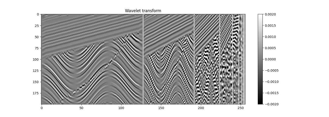
As a comparison we also compute the Seislet transform fixing slopes to zero. This way we turn the Seislet tranform into a basic 1d Wavelet transform performed over the spatial axis.

Wop = pylops.signalprocessing.Seislet(np.zeros_like(slope.T),
                                      sampling=(dx, dt))
dwt = Wop * d.ravel()
dwt = dwt.reshape(nx, nt)

plt.figure(figsize=(14, 5))
plt.imshow(dwt.T, cmap='gray', vmin=-clip, vmax=clip)
for level in levels_cum:
    plt.axvline(level-0.5, color='w')
plt.title('Wavelet transform')
plt.colorbar()
plt.axis('tight')

Out:

(-0.5, 255.5, 199.5, -0.5)

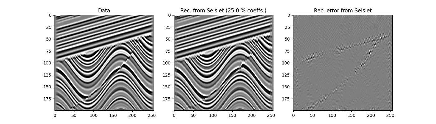
Finally we evaluate the compression capabilities of the Seislet transform. We zero-out all coefficients at the first two fine resolutions and keep those at coarser resolutions. We perform the inverse Seislet transform and asses the compression error.

seis1 = seis.copy()
seis1[:levels_cum[1]] = 0
drec1 = Sop.inverse(seis1.ravel())
drec1 = drec1.reshape(nx, nt)

fig, axs = plt.subplots(1, 3, figsize=(14, 4))
axs[0].imshow(d.T, cmap='gray', vmin=-clip, vmax=clip)
axs[0].set_title('Data')
axs[0].axis('tight')
axs[1].imshow(drec1.T, cmap='gray', vmin=-clip, vmax=clip)
axs[1].set_title('Rec. from Seislet (%.1f %% coeffs.)' %
                 (100 * (nx - levels_cum[1]) / nx))
axs[1].axis('tight')
axs[2].imshow(d.T - drec1.T, cmap='gray', vmin=-clip, vmax=clip)
axs[2].set_title('Rec. error from Seislet')
axs[2].axis('tight')

Out:

(-0.5, 255.5, 199.5, -0.5)

To conclude it is worth noting that the Seislet transform, opposite to the Wavelet transform, is not an orthogonal transformation: in other words, its adjoint and inverse are not equivalent. While we have used it the forward and inverse transformations, when used as part of a linear operator to be inverted the Seislet transform requires the forward-adjoint pair that is implemented in PyLops and passes the dot-test as shown below

pylops.utils.dottest(Sop, nt*nx, nt*nx, verb=True)

Out:

Dot test passed, v^T(Opu)=-166.650972 - u^T(Op^Tv)=-166.650972

True