1D Smoothing

This example shows how to use the pylops.Smoothing1D operator to smooth an input signal along a given axis.

Derivative (or roughening) operators are generally used regularization in inverse problems. Smoothing has the opposite effect of roughening and it can be employed as preconditioning in inverse problems.

A smoothing operator is a simple compact filter on lenght \(n_{smooth}\) and each elements is equal to \(1/n_{smooth}\).

import numpy as np
import matplotlib.pyplot as plt

import pylops

plt.close('all')

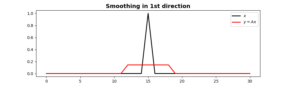
Define the input parameters: number of samples of input signal (N) and lenght of the smoothing filter regression coefficients (\(n_{smooth}\)). In this first case the input signal is one at the center and zero elsewhere.

N = 31
nsmooth = 7
x = np.zeros(N)
x[int(N/2)] = 1

Sop = pylops.Smoothing1D(nsmooth=nsmooth, dims=[N], dtype='float32')

y = Sop*x
xadj = Sop.H*y

fig, ax = plt.subplots(1, 1, figsize=(10, 3))
ax.plot(x, 'k', lw=2, label=r'$x$')
ax.plot(y, 'r', lw=2, label=r'$y=Ax$')
ax.set_title('Smoothing in 1st direction', fontsize=14, fontweight='bold')
ax.legend()

Out:

<matplotlib.legend.Legend object at 0x7f835c432048>

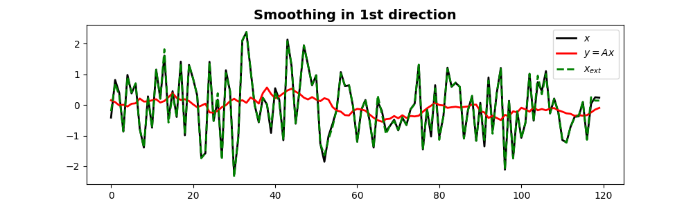
Let’s repeat the same exercise with a random signal as input. After applying smoothing, we will also try to invert it.

N = 120
nsmooth = 13
x = np.random.normal(0, 1, N)
Sop = pylops.Smoothing1D(nsmooth=13, dims=(N), dtype='float32')

y = Sop*x
xest = Sop/y

fig, ax = plt.subplots(1, 1, figsize=(10, 3))
ax.plot(x, 'k', lw=2, label=r'$x$')
ax.plot(y, 'r', lw=2, label=r'$y=Ax$')
ax.plot(xest, '--g', lw=2, label=r'$x_{ext}$')
ax.set_title('Smoothing in 1st direction',
             fontsize=14, fontweight='bold')
ax.legend()

Out:

<matplotlib.legend.Legend object at 0x7f8359e7a438>

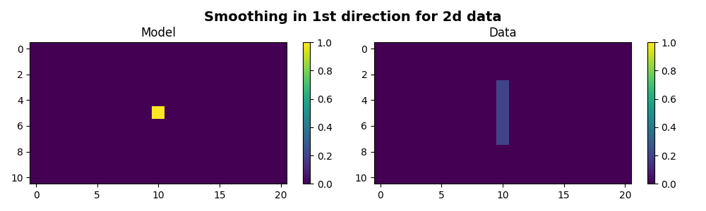
Finally we show that the same operator can be applied to multi-dimensional data along a chosen axis.

A = np.zeros((11, 21))
A[5, 10] = 1

Sop = pylops.Smoothing1D(nsmooth=5, dims=(11, 21), dir=0, dtype='float64')
B = np.reshape(Sop*np.ndarray.flatten(A), (11, 21))

fig, axs = plt.subplots(1, 2, figsize=(10, 3))
fig.suptitle('Smoothing in 1st direction for 2d data', fontsize=14,
             fontweight='bold', y=0.95)
im = axs[0].imshow(A, interpolation='nearest', vmin=0, vmax=1)
axs[0].axis('tight')
axs[0].set_title('Model')
plt.colorbar(im, ax=axs[0])
im = axs[1].imshow(B, interpolation='nearest', vmin=0, vmax=1)
axs[1].axis('tight')
axs[1].set_title('Data')
plt.colorbar(im, ax=axs[1])
plt.tight_layout()
plt.subplots_adjust(top=0.8)