16. CT Scan Imaging

This tutorial considers a very well-known inverse problem from the field of medical imaging.

We will be using the pylops.signalprocessing.Radon2D operator to model a sinogram, which is a graphic representation of the raw data obtained from a CT scan. The sinogram is further inverted using both a L2 solver and a TV-regularized solver like Split-Bregman.

# sphinx_gallery_thumbnail_number = 2
import numpy as np
import matplotlib.pyplot as plt
import pylops

from numba import jit

plt.close('all')
np.random.seed(10)

Let’s start by loading the Shepp-Logan phantom model. We can then construct the sinogram by providing a custom-made function to the pylops.signalprocessing.Radon2D that samples parametric curves of such a type:

\[t(r,\theta; x) = tan(90-\theta)*x + r/sin(\theta)\]

where \(\theta\) is the angle between the x-axis (\(x\)) and the perpendicular to the summation line and \(r\) is the distance from the origin of the summation line.

@jit(nopython=True)
def radoncurve(x, r, theta):
    return (r - ny//2)/(np.sin(np.deg2rad(theta))+1e-15) + np.tan(np.deg2rad(90 - theta))*x  + ny//2

x = np.load('../testdata/optimization/shepp_logan_phantom.npy')
x = x / x.max()
ny, nx = x.shape

ntheta = 150
theta = np.linspace(0., 180., ntheta, endpoint=False)

RLop = \
    pylops.signalprocessing.Radon2D(np.arange(ny), np.arange(nx),
                                    theta, kind=radoncurve,
                                    centeredh=True, interp=False,
                                    engine='numba', dtype='float64')

y = RLop.H * x.T.ravel()
y = y.reshape(ntheta, ny).T

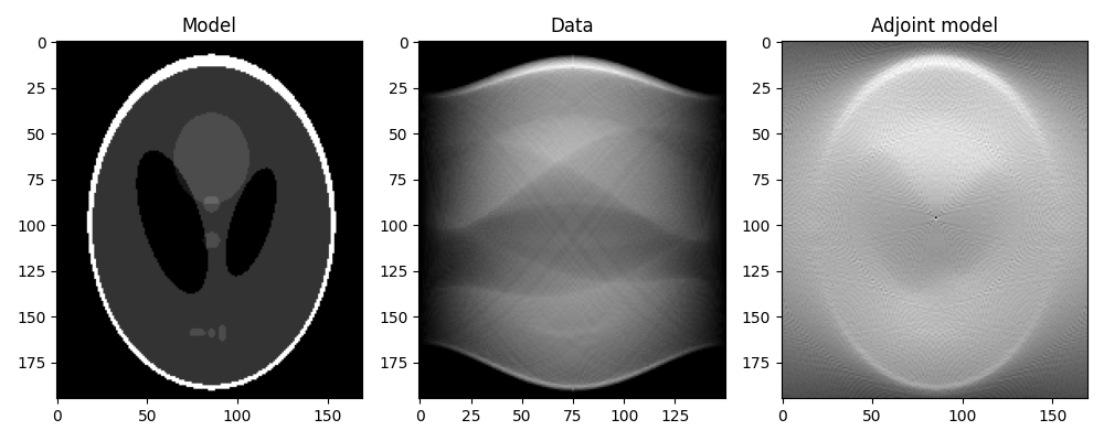
We can now first perform the adjoint, which in the medical imaging literature is also referred to as back-projection.

This is the first step of a common reconstruction technique, named filtered back-projection, which simply applies a correction filter in the frequency domain to the adjoint model.

xrec = RLop*y.T.ravel()
xrec = xrec.reshape(nx, ny).T

fig, axs = plt.subplots(1, 3, figsize=(10, 4))
axs[0].imshow(x, vmin=0, vmax=1, cmap='gray')
axs[0].set_title('Model')
axs[0].axis('tight')
axs[1].imshow(y, cmap='gray')
axs[1].set_title('Data')
axs[1].axis('tight')
axs[2].imshow(xrec, cmap='gray')
axs[2].set_title('Adjoint model')
axs[2].axis('tight')
fig.tight_layout()

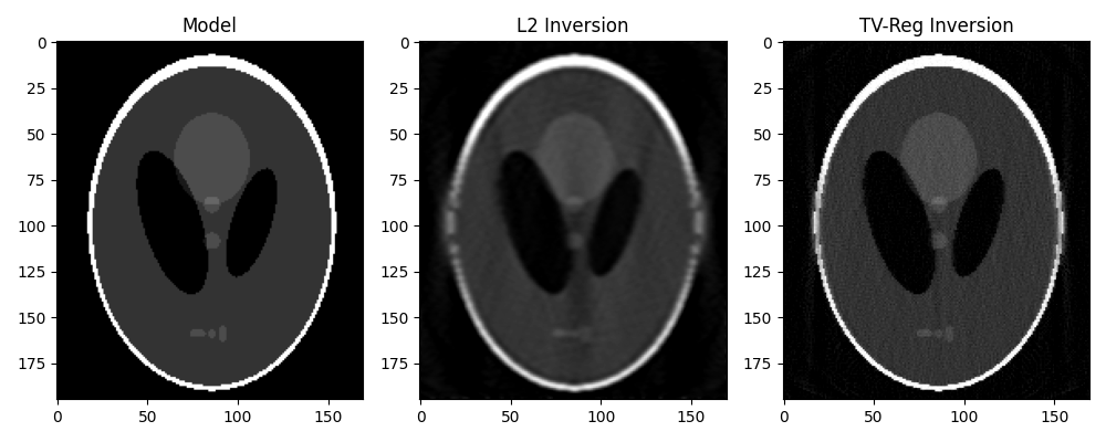
Finally we take advantage of our different solvers and try to invert the modelling operator both in a least-squares sense and using TV-reg.

Dop = [
    pylops.FirstDerivative(ny * nx, dims=(nx, ny), dir=0, edge=True, dtype=np.float),
    pylops.FirstDerivative(ny * nx, dims=(nx, ny), dir=1, edge=True, dtype=np.float)]
D2op = pylops.Laplacian(dims=(nx, ny), edge=True, dtype=np.float)

# L2
xinv_sm = \
    pylops.optimization.leastsquares.RegularizedInversion(RLop.H,
                                                          [D2op],
                                                          y.T.flatten(),
                                                          epsRs=[1e1],
                                                          **dict(iter_lim=20))
xinv_sm = np.real(xinv_sm.reshape(nx, ny)).T

# TV
mu = 1.5
lamda = [1., 1.]
niter = 3
niterinner = 4

xinv, niter = pylops.optimization.sparsity.SplitBregman(RLop.H, Dop, y.T.flatten(), niter, niterinner,
                           mu=mu, epsRL1s=lamda, tol=1e-4, tau=1., show=False,
                           **dict(iter_lim=20, damp=1e-2))
xinv = np.real(xinv.reshape(nx, ny)).T

fig, axs = plt.subplots(1, 3, figsize=(10, 4))
axs[0].imshow(x, vmin=0, vmax=1, cmap='gray')
axs[0].set_title('Model')
axs[0].axis('tight')
axs[1].imshow(xinv_sm, vmin=0, vmax=1, cmap='gray')
axs[1].set_title('L2 Inversion')
axs[1].axis('tight')
axs[2].imshow(xinv, vmin=0, vmax=1, cmap='gray')
axs[2].set_title('TV-Reg Inversion')
axs[2].axis('tight')
fig.tight_layout()