pylops.waveeqprocessing.UpDownComposition2D
-
pylops.waveeqprocessing.UpDownComposition2D(nt, nr, dt, dr, rho, vel, nffts=(None, None), critical=100.0, ntaper=10, scaling=1.0, dtype='complex128')[source]¶ 2D Up-down wavefield composition.
Apply multi-component seismic wavefield composition from its up- and down-going constituents. The input model required by the operator should be created by flattening the separated wavefields of size \(\lbrack n_r \times n_t \rbrack\) concatenated along the spatial axis.
Similarly, the data is also a flattened concatenation of pressure and vertical particle velocity wavefields.
Parameters: - nt :
int Number of samples along the time axis
- nr :
int Number of samples along the receiver axis
- dt :
float Sampling along the time axis
- dr :
float Sampling along the receiver array
- rho :
float Density along the receiver array (must be constant)
- vel :
float Velocity along the receiver array (must be constant)
- nffts :
tuple, optional Number of samples along the wavenumber and frequency axes
- critical :
float, optional Percentage of angles to retain in obliquity factor. For example, if
critical=100only angles below the critical angle \(|k_x| < \frac{f(k_x)}{vel}\) will be retained will be retained- ntaper :
float, optional Number of samples of taper applied to obliquity factor around critical angle
- scaling :
float, optional Scaling to apply to the operator (see Notes for more details)
- dtype :
str, optional Type of elements in input array.
Returns: - UDop :
pylops.LinearOperator Up-down wavefield composition operator
See also
UpDownComposition3D- 3D Wavefield composition
WavefieldDecomposition- Wavefield decomposition
Notes
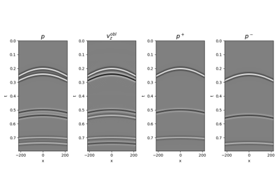
Multi-component seismic data (\(p(x, t)\) and \(v_z(x, t)\)) can be synthesized in the frequency-wavenumber domain as the superposition of the up- and downgoing constituents of the pressure wavefield (\(p^-(x, t)\) and \(p^+(x, t)\)) as follows [1]:
\[\begin{split}\begin{bmatrix} \mathbf{p}(k_x, \omega) \\ \mathbf{v_z}(k_x, \omega) \end{bmatrix} = \begin{bmatrix} 1 & 1 \\ \frac{k_z}{\omega \rho} & - \frac{k_z}{\omega \rho} \\ \end{bmatrix} \begin{bmatrix} \mathbf{p^+}(k_x, \omega) \\ \mathbf{p^-}(k_x, \omega) \end{bmatrix}\end{split}\]where the vertical wavenumber \(k_z\) is defined as \(k_z=\sqrt{\omega^2/c^2 - k_x^2}\).
We can write the entire composition process in a compact matrix-vector notation as follows:
\[\begin{split}\begin{bmatrix} \mathbf{p} \\ s*\mathbf{v_z} \end{bmatrix} = \begin{bmatrix} \mathbf{F} & 0 \\ 0 & s*\mathbf{F} \end{bmatrix} \begin{bmatrix} \mathbf{I} & \mathbf{I} \\ \mathbf{W}^+ & \mathbf{W}^- \end{bmatrix} \begin{bmatrix} \mathbf{F}^H & 0 \\ 0 & \mathbf{F}^H \end{bmatrix} \mathbf{p^{\pm}}\end{split}\]where \(\mathbf{F}\) is the 2-dimensional FFT (
pylops.signalprocessing.FFT2), \(\mathbf{W}^\pm\) are weighting matrices which contain the scalings \(\pm \frac{k_z}{\omega \rho}\) implemented viapylops.basicprocessing.Diagonal, and \(s\) is a scaling factor that is applied to both the particle velocity data and to the operator has shown above. Such a scaling is required to balance out the different dynamic range of pressure and particle velocity when solving the wavefield separation problem as an inverse problem.As the operator is effectively obtained by chaining basic PyLops operators the adjoint is automatically implemented for this operator.
[1] Wapenaar, K. “Reciprocity properties of one-way propagators”, Geophysics, vol. 63, pp. 1795-1798. 1998. - nt :