pylops.optimization.basic.lsqr
- pylops.optimization.basic.lsqr(Op, y, x0=None, damp=0.0, atol=1e-08, btol=1e-08, conlim=100000000.0, niter=10, calc_var=True, show=False, itershow=[10, 10, 10], callback=None)[source]
LSQR
Solve an overdetermined system of equations given an operator
Opand datayusing LSQR iterations.\[\DeclareMathOperator{\cond}{cond}\]- Parameters
- Op
pylops.LinearOperator Operator to invert of size \([N \times M]\)
- y
np.ndarray Data of size \([N \times 1]\)
- x0
np.ndarray, optional Initial guess of size \([M \times 1]\)
- damp
float, optional Damping coefficient
- atol, btol
float, optional Stopping tolerances. If both are 1.0e-9, the final residual norm should be accurate to about 9 digits. (The solution will usually have fewer correct digits, depending on \(\cond(\mathbf{Op})\) and the size of
damp.)- conlim
float, optional Stopping tolerance on \(\cond(\mathbf{Op})\) exceeds
conlim. For square,conlimcould be as large as 1.0e+12. For least-squares problems,conlimshould be less than 1.0e+8. Maximum precision can be obtained by settingatol = btol = conlim = 0, but the number of iterations may then be excessive.- niter
int, optional Number of iterations
- calc_var
bool, optional Estimate diagonals of \((\mathbf{Op}^H\mathbf{Op} + \epsilon^2\mathbf{I})^{-1}\).
- show
bool, optional Display iterations log
- itershow
list, optional Display set log for the first N1 steps, last N2 steps, and every N3 steps in between where N1, N2, N3 are the three element of the list.
- callback
callable, optional Function with signature (
callback(x)) to call after each iteration wherexis the current model vector
- Op
- Returns
- x
np.ndarray Estimated model of size \([M \times 1]\)
- istop
int Gives the reason for termination
0means the exact solution is \(\mathbf{x}=0\)1means \(\mathbf{x}\) is an approximate solution to \(\mathbf{y} = \mathbf{Op}\,\mathbf{x}\)2means \(\mathbf{x}\) approximately solves the least-squares problem3means the estimate of \(\cond(\overline{\mathbf{Op}})\) has exceededconlim4means \(\mathbf{y} - \mathbf{Op}\,\mathbf{x}\) is small enough for this machine5means the least-squares solution is good enough for this machine6means \(\cond(\overline{\mathbf{Op}})\) seems to be too large for this machine7means the iteration limit has been reached- r1norm
float \(||\mathbf{r}||_2^2\), where \(\mathbf{r} = \mathbf{y} - \mathbf{Op}\,\mathbf{x}\)
- r2norm
float \(\sqrt{\mathbf{r}^T\mathbf{r} + \epsilon^2 \mathbf{x}^T\mathbf{x}}\). Equal to
r1normif \(\epsilon=0\)- anorm
float Estimate of Frobenius norm of \(\overline{\mathbf{Op}} = [\mathbf{Op} \; \epsilon \mathbf{I}]\)
- acond
float Estimate of \(\cond(\overline{\mathbf{Op}})\)
- arnorm
float Estimate of norm of \(\cond(\mathbf{Op}^H\mathbf{r}- \epsilon^2\mathbf{x})\)
- var
float Diagonals of \((\mathbf{Op}^H\mathbf{Op})^{-1}\) (if
damp=0) or more generally \((\mathbf{Op}^H\mathbf{Op} + \epsilon^2\mathbf{I})^{-1}\).- cost
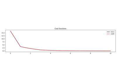
numpy.ndarray, optional History of r1norm through iterations
- x
Notes