Note
Click here to download the full example code
08. Pre-stack (AVO) inversion
Pre-stack inversion represents one step beyond post-stack inversion in that not only the profile of acoustic impedance can be inferred from seismic data, rather a set of elastic parameters is estimated from pre-stack data (i.e., angle gathers) using the information contained in the so-called AVO (amplitude versus offset) response. Such elastic parameters represent vital information for more sophisticated geophysical subsurface characterization than it would be possible to achieve working with post-stack seismic data.
In this tutorial, the pylops.avo.prestack.PrestackLinearModelling
operator is used for modelling of both 1d and 2d synthetic pre-stack seismic
data using 1d profiles or 2d models of different subsurface elastic parameters
(P-wave velocity, S-wave velocity, and density) as input.
where \(\mathbf{m}(t)=[V_P(t), V_S(t), \rho(t)]\) is a vector containing three elastic parameters at time \(t\), \(G_i(t, \theta)\) are the coefficients of the AVO parametrization used to model pre-stack data and \(w(t)\) is the time domain seismic wavelet. In compact form:
where \(\mathbf{W}\) is a convolution operator, \(\mathbf{G}\) is
the AVO modelling operator, \(\mathbf{D}\) is a block-diagonal
derivative operator, and \(\mathbf{m}\) is the input model.
Subsequently the elastic parameters are estimated via the
pylops.avo.prestack.PrestackInversion module.
Once again, a two-steps inversion strategy can also be used to deal
with the case of noisy data.
import matplotlib.pyplot as plt
import numpy as np
from scipy.signal import filtfilt

import pylops
from pylops.utils.wavelets import ricker

plt.close("all")
np.random.seed(0)
Let’s start with a 1d example. A synthetic profile of acoustic impedance
is created and data is modelled using both the dense and linear operator
version of pylops.avo.prestack.PrestackLinearModelling operator
# sphinx_gallery_thumbnail_number = 5

# model
nt0 = 301
dt0 = 0.004

t0 = np.arange(nt0) * dt0
vp = 1200 + np.arange(nt0) + filtfilt(np.ones(5) / 5.0, 1, np.random.normal(0, 80, nt0))
vs = 600 + vp / 2 + filtfilt(np.ones(5) / 5.0, 1, np.random.normal(0, 20, nt0))
rho = 1000 + vp + filtfilt(np.ones(5) / 5.0, 1, np.random.normal(0, 30, nt0))
vp[131:] += 500
vs[131:] += 200
rho[131:] += 100
vsvp = 0.5
m = np.stack((np.log(vp), np.log(vs), np.log(rho)), axis=1)

# background model
nsmooth = 50
mback = filtfilt(np.ones(nsmooth) / float(nsmooth), 1, m, axis=0)

# angles
ntheta = 21
thetamin, thetamax = 0, 40
theta = np.linspace(thetamin, thetamax, ntheta)

# wavelet
ntwav = 41
wav = ricker(t0[: ntwav // 2 + 1], 15)[0]

# lop
PPop = pylops.avo.prestack.PrestackLinearModelling(
    wav, theta, vsvp=vsvp, nt0=nt0, linearization="akirich"
)

# dense
PPop_dense = pylops.avo.prestack.PrestackLinearModelling(
    wav, theta, vsvp=vsvp, nt0=nt0, linearization="akirich", explicit=True
)

# data lop
dPP = PPop * m.ravel()
dPP = dPP.reshape(nt0, ntheta)

# data dense
dPP_dense = PPop_dense * m.T.ravel()
dPP_dense = dPP_dense.reshape(ntheta, nt0).T

# noisy data
dPPn_dense = dPP_dense + np.random.normal(0, 1e-2, dPP_dense.shape)
We can now invert our data and retrieve elastic profiles for both noise-free
and noisy data using pylops.avo.prestack.PrestackInversion.
# dense
minv_dense, dPP_dense_res = pylops.avo.prestack.PrestackInversion(
    dPP_dense,
    theta,
    wav,
    m0=mback,
    linearization="akirich",
    explicit=True,
    returnres=True,
    **dict(cond=1e-10)
)

# lop
minv, dPP_res = pylops.avo.prestack.PrestackInversion(
    dPP,
    theta,
    wav,
    m0=mback,
    linearization="akirich",
    explicit=False,
    returnres=True,
    **dict(damp=1e-10, iter_lim=2000)
)

# dense noisy
minv_dense_noise, dPPn_dense_res = pylops.avo.prestack.PrestackInversion(
    dPPn_dense,
    theta,
    wav,
    m0=mback,
    linearization="akirich",
    explicit=True,
    returnres=True,
    **dict(cond=1e-1)
)

# lop noisy (with vertical smoothing)
minv_noise, dPPn_res = pylops.avo.prestack.PrestackInversion(
    dPPn_dense,
    theta,
    wav,
    m0=mback,
    linearization="akirich",
    explicit=False,
    epsR=5e-1,
    returnres=True,
    **dict(damp=1e-1, iter_lim=100)
)
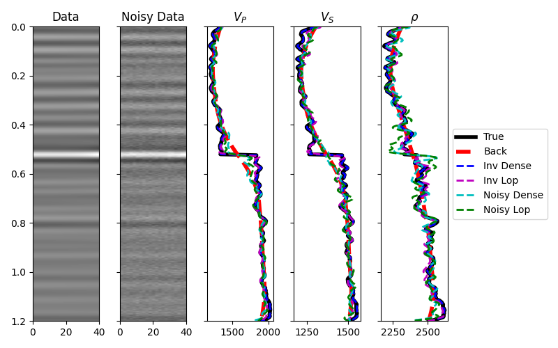
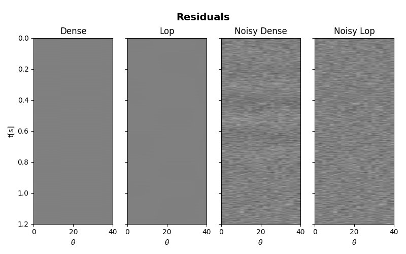
The data, inverted models and residuals are now displayed.
# data and model
fig, (axd, axdn, axvp, axvs, axrho) = plt.subplots(1, 5, figsize=(8, 5), sharey=True)
axd.imshow(
    dPP_dense,
    cmap="gray",
    extent=(theta[0], theta[-1], t0[-1], t0[0]),
    vmin=-np.abs(dPP_dense).max(),
    vmax=np.abs(dPP_dense).max(),
)
axd.set_title("Data")
axd.axis("tight")
axdn.imshow(
    dPPn_dense,
    cmap="gray",
    extent=(theta[0], theta[-1], t0[-1], t0[0]),
    vmin=-np.abs(dPP_dense).max(),
    vmax=np.abs(dPP_dense).max(),
)
axdn.set_title("Noisy Data")
axdn.axis("tight")
axvp.plot(vp, t0, "k", lw=4, label="True")
axvp.plot(np.exp(mback[:, 0]), t0, "--r", lw=4, label="Back")
axvp.plot(np.exp(minv_dense[:, 0]), t0, "--b", lw=2, label="Inv Dense")
axvp.plot(np.exp(minv[:, 0]), t0, "--m", lw=2, label="Inv Lop")
axvp.plot(np.exp(minv_dense_noise[:, 0]), t0, "--c", lw=2, label="Noisy Dense")
axvp.plot(np.exp(minv_noise[:, 0]), t0, "--g", lw=2, label="Noisy Lop")
axvp.set_title(r"$V_P$")
axvs.plot(vs, t0, "k", lw=4, label="True")
axvs.plot(np.exp(mback[:, 1]), t0, "--r", lw=4, label="Back")
axvs.plot(np.exp(minv_dense[:, 1]), t0, "--b", lw=2, label="Inv Dense")
axvs.plot(np.exp(minv[:, 1]), t0, "--m", lw=2, label="Inv Lop")
axvs.plot(np.exp(minv_dense_noise[:, 1]), t0, "--c", lw=2, label="Noisy Dense")
axvs.plot(np.exp(minv_noise[:, 1]), t0, "--g", lw=2, label="Noisy Lop")
axvs.set_title(r"$V_S$")
axrho.plot(rho, t0, "k", lw=4, label="True")
axrho.plot(np.exp(mback[:, 2]), t0, "--r", lw=4, label="Back")
axrho.plot(np.exp(minv_dense[:, 2]), t0, "--b", lw=2, label="Inv Dense")
axrho.plot(np.exp(minv[:, 2]), t0, "--m", lw=2, label="Inv Lop")
axrho.plot(np.exp(minv_dense_noise[:, 2]), t0, "--c", lw=2, label="Noisy Dense")
axrho.plot(np.exp(minv_noise[:, 2]), t0, "--g", lw=2, label="Noisy Lop")
axrho.set_title(r"$\rho$")
axrho.legend(loc="center left", bbox_to_anchor=(1, 0.5))
axd.axis("tight")
plt.tight_layout()

# residuals
fig, axs = plt.subplots(1, 4, figsize=(8, 5), sharey=True)
fig.suptitle("Residuals", fontsize=14, fontweight="bold", y=0.95)
im = axs[0].imshow(
    dPP_dense_res,
    cmap="gray",
    extent=(theta[0], theta[-1], t0[-1], t0[0]),
    vmin=-0.1,
    vmax=0.1,
)
axs[0].set_title("Dense")
axs[0].set_xlabel(r"$\theta$")
axs[0].set_ylabel("t[s]")
axs[0].axis("tight")
axs[1].imshow(
    dPP_res,
    cmap="gray",
    extent=(theta[0], theta[-1], t0[-1], t0[0]),
    vmin=-0.1,
    vmax=0.1,
)
axs[1].set_title("Lop")
axs[1].set_xlabel(r"$\theta$")
axs[1].axis("tight")
axs[2].imshow(
    dPPn_dense_res,
    cmap="gray",
    extent=(theta[0], theta[-1], t0[-1], t0[0]),
    vmin=-0.1,
    vmax=0.1,
)
axs[2].set_title("Noisy Dense")
axs[2].set_xlabel(r"$\theta$")
axs[2].axis("tight")
axs[3].imshow(
    dPPn_res,
    cmap="gray",
    extent=(theta[0], theta[-1], t0[-1], t0[0]),
    vmin=-0.1,
    vmax=0.1,
)
axs[3].set_title("Noisy Lop")
axs[3].set_xlabel(r"$\theta$")
axs[3].axis("tight")
plt.tight_layout()
plt.subplots_adjust(top=0.85)
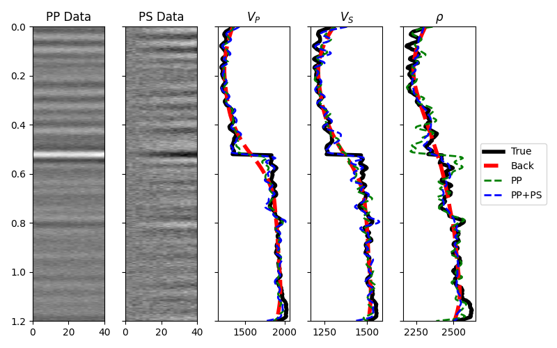
Finally before moving to the 2d example, we consider the case when both PP and PS data are available. A joint PP-PS inversion can be easily solved as follows.
PSop = pylops.avo.prestack.PrestackLinearModelling(
    2 * wav, theta, vsvp=vsvp, nt0=nt0, linearization="ps"
)
PPPSop = pylops.VStack((PPop, PSop))

# data
dPPPS = PPPSop * m.ravel()
dPPPS = dPPPS.reshape(2, nt0, ntheta)

dPPPSn = dPPPS + np.random.normal(0, 1e-2, dPPPS.shape)

# Invert
minvPPSP, dPPPS_res = pylops.avo.prestack.PrestackInversion(
    dPPPS,
    theta,
    [wav, 2 * wav],
    m0=mback,
    linearization=["fatti", "ps"],
    epsR=5e-1,
    returnres=True,
    **dict(damp=1e-1, iter_lim=100)
)

# Data and model
fig, (axd, axdn, axvp, axvs, axrho) = plt.subplots(1, 5, figsize=(8, 5), sharey=True)
axd.imshow(
    dPPPSn[0],
    cmap="gray",
    extent=(theta[0], theta[-1], t0[-1], t0[0]),
    vmin=-np.abs(dPPPSn[0]).max(),
    vmax=np.abs(dPPPSn[0]).max(),
)
axd.set_title("PP Data")
axd.axis("tight")
axdn.imshow(
    dPPPSn[1],
    cmap="gray",
    extent=(theta[0], theta[-1], t0[-1], t0[0]),
    vmin=-np.abs(dPPPSn[1]).max(),
    vmax=np.abs(dPPPSn[1]).max(),
)
axdn.set_title("PS Data")
axdn.axis("tight")
axvp.plot(vp, t0, "k", lw=4, label="True")
axvp.plot(np.exp(mback[:, 0]), t0, "--r", lw=4, label="Back")
axvp.plot(np.exp(minv_noise[:, 0]), t0, "--g", lw=2, label="PP")
axvp.plot(np.exp(minvPPSP[:, 0]), t0, "--b", lw=2, label="PP+PS")
axvp.set_title(r"$V_P$")
axvs.plot(vs, t0, "k", lw=4, label="True")
axvs.plot(np.exp(mback[:, 1]), t0, "--r", lw=4, label="Back")
axvs.plot(np.exp(minv_noise[:, 1]), t0, "--g", lw=2, label="PP")
axvs.plot(np.exp(minvPPSP[:, 1]), t0, "--b", lw=2, label="PP+PS")
axvs.set_title(r"$V_S$")
axrho.plot(rho, t0, "k", lw=4, label="True")
axrho.plot(np.exp(mback[:, 2]), t0, "--r", lw=4, label="Back")
axrho.plot(np.exp(minv_noise[:, 2]), t0, "--g", lw=2, label="PP")
axrho.plot(np.exp(minvPPSP[:, 2]), t0, "--b", lw=2, label="PP+PS")
axrho.set_title(r"$\rho$")
axrho.legend(loc="center left", bbox_to_anchor=(1, 0.5))
axd.axis("tight")
plt.tight_layout()
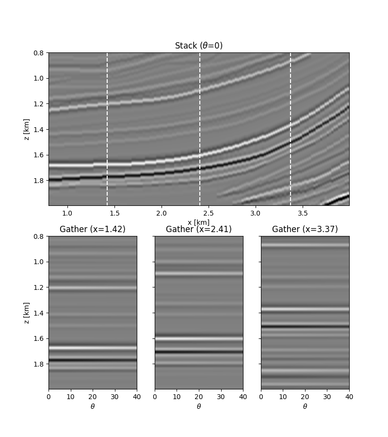
We move now to a 2d example. First of all the model is loaded and data generated.
# model
inputfile = "../testdata/avo/poststack_model.npz"

model = np.load(inputfile)
x, z = model["x"][::6] / 1000.0, model["z"][:300] / 1000.0
nx, nz = len(x), len(z)
m = 1000 * model["model"][:300, ::6]

mvp = m.copy()
mvs = m / 2
mrho = m / 3 + 300
m = np.log(np.stack((mvp, mvs, mrho), axis=1))

# smooth model
nsmoothz, nsmoothx = 30, 25
mback = filtfilt(np.ones(nsmoothz) / float(nsmoothz), 1, m, axis=0)
mback = filtfilt(np.ones(nsmoothx) / float(nsmoothx), 1, mback, axis=2)

# dense operator
PPop_dense = pylops.avo.prestack.PrestackLinearModelling(
    wav,
    theta,
    vsvp=vsvp,
    nt0=nz,
    spatdims=(nx,),
    linearization="akirich",
    explicit=True,
)

# lop operator
PPop = pylops.avo.prestack.PrestackLinearModelling(
    wav, theta, vsvp=vsvp, nt0=nz, spatdims=(nx,), linearization="akirich"
)

# data
dPP = PPop_dense * m.swapaxes(0, 1).ravel()
dPP = dPP.reshape(ntheta, nz, nx).swapaxes(0, 1)
dPPn = dPP + np.random.normal(0, 5e-2, dPP.shape)
Finally we perform the same 4 different inversions as in the post-stack tutorial (see 07. Post-stack inversion for more details).
# dense inversion with noise-free data
minv_dense = pylops.avo.prestack.PrestackInversion(
    dPP, theta, wav, m0=mback, explicit=True, simultaneous=False
)

# dense inversion with noisy data
minv_dense_noisy = pylops.avo.prestack.PrestackInversion(
    dPPn, theta, wav, m0=mback, explicit=True, epsI=4e-2, simultaneous=False
)

# spatially regularized lop inversion with noisy data
minv_lop_reg = pylops.avo.prestack.PrestackInversion(
    dPPn,
    theta,
    wav,
    m0=minv_dense_noisy,
    explicit=False,
    epsR=1e1,
    **dict(damp=np.sqrt(1e-4), iter_lim=20)
)

# blockiness promoting inversion with noisy data
minv_blocky = pylops.avo.prestack.PrestackInversion(
    dPPn,
    theta,
    wav,
    m0=mback,
    explicit=False,
    epsR=0.4,
    epsRL1=0.1,
    **dict(mu=0.1, niter_outer=3, niter_inner=3, iter_lim=5, damp=1e-3)
)
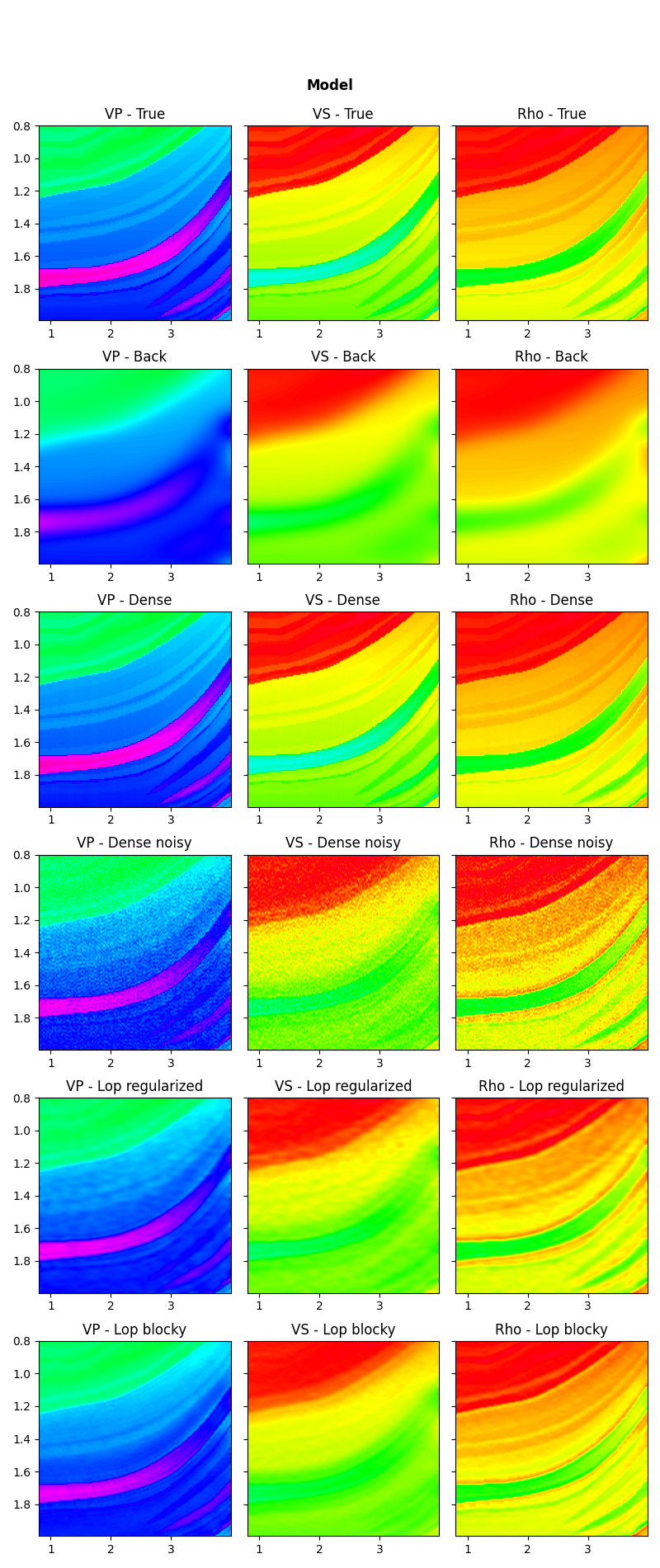
Let’s now visualize the inverted elastic parameters for the different scenarios
def plotmodel(
axs,
m,
x,
z,
vmin,
vmax,
params=("VP", "VS", "Rho"),
cmap="gist_rainbow",
title=None,
):
"""Quick visualization of model"""
for ip, param in enumerate(params):
axs[ip].imshow(
m[:, ip], extent=(x[0], x[-1], z[-1], z[0]), vmin=vmin, vmax=vmax, cmap=cmap
)
axs[ip].set_title("%s - %s" % (param, title))
axs[ip].axis("tight")
plt.setp(axs[1].get_yticklabels(), visible=False)
plt.setp(axs[2].get_yticklabels(), visible=False)
# data
fig = plt.figure(figsize=(8, 9))
ax1 = plt.subplot2grid((2, 3), (0, 0), colspan=3)
ax2 = plt.subplot2grid((2, 3), (1, 0))
ax3 = plt.subplot2grid((2, 3), (1, 1), sharey=ax2)
ax4 = plt.subplot2grid((2, 3), (1, 2), sharey=ax2)
ax1.imshow(
dPP[:, 0], cmap="gray", extent=(x[0], x[-1], z[-1], z[0]), vmin=-0.4, vmax=0.4
)
ax1.vlines(
[x[nx // 5], x[nx // 2], x[4 * nx // 5]],
ymin=z[0],
ymax=z[-1],
colors="w",
linestyles="--",
)
ax1.set_xlabel("x [km]")
ax1.set_ylabel("z [km]")
ax1.set_title(r"Stack ($\theta$=0)")
ax1.axis("tight")
ax2.imshow(
dPP[:, :, nx // 5],
cmap="gray",
extent=(theta[0], theta[-1], z[-1], z[0]),
vmin=-0.4,
vmax=0.4,
)
ax2.set_xlabel(r"$\theta$")
ax2.set_ylabel("z [km]")
ax2.set_title(r"Gather (x=%.2f)" % x[nx // 5])
ax2.axis("tight")
ax3.imshow(
dPP[:, :, nx // 2],
cmap="gray",
extent=(theta[0], theta[-1], z[-1], z[0]),
vmin=-0.4,
vmax=0.4,
)
ax3.set_xlabel(r"$\theta$")
ax3.set_title(r"Gather (x=%.2f)" % x[nx // 2])
ax3.axis("tight")
ax4.imshow(
dPP[:, :, 4 * nx // 5],
cmap="gray",
extent=(theta[0], theta[-1], z[-1], z[0]),
vmin=-0.4,
vmax=0.4,
)
ax4.set_xlabel(r"$\theta$")
ax4.set_title(r"Gather (x=%.2f)" % x[4 * nx // 5])
ax4.axis("tight")
plt.setp(ax3.get_yticklabels(), visible=False)
plt.setp(ax4.get_yticklabels(), visible=False)
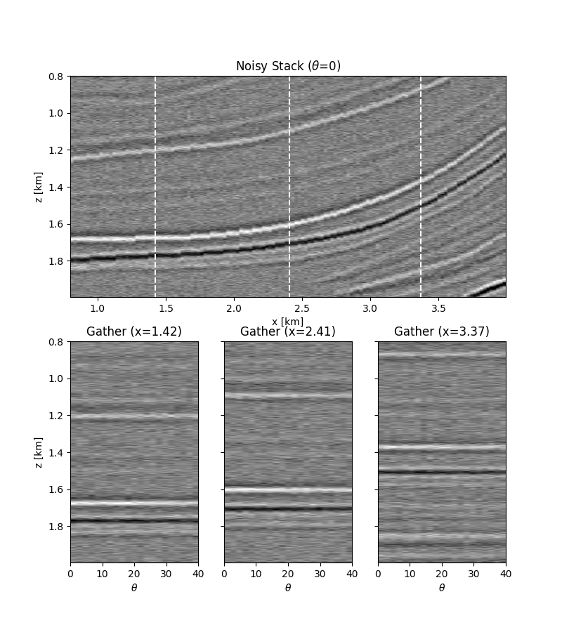
# noisy data
fig = plt.figure(figsize=(8, 9))
ax1 = plt.subplot2grid((2, 3), (0, 0), colspan=3)
ax2 = plt.subplot2grid((2, 3), (1, 0))
ax3 = plt.subplot2grid((2, 3), (1, 1), sharey=ax2)
ax4 = plt.subplot2grid((2, 3), (1, 2), sharey=ax2)
ax1.imshow(
dPPn[:, 0], cmap="gray", extent=(x[0], x[-1], z[-1], z[0]), vmin=-0.4, vmax=0.4
)
ax1.vlines(
[x[nx // 5], x[nx // 2], x[4 * nx // 5]],
ymin=z[0],
ymax=z[-1],
colors="w",
linestyles="--",
)
ax1.set_xlabel("x [km]")
ax1.set_ylabel("z [km]")
ax1.set_title(r"Noisy Stack ($\theta$=0)")
ax1.axis("tight")
ax2.imshow(
dPPn[:, :, nx // 5],
cmap="gray",
extent=(theta[0], theta[-1], z[-1], z[0]),
vmin=-0.4,
vmax=0.4,
)
ax2.set_xlabel(r"$\theta$")
ax2.set_ylabel("z [km]")
ax2.set_title(r"Gather (x=%.2f)" % x[nx // 5])
ax2.axis("tight")
ax3.imshow(
dPPn[:, :, nx // 2],
cmap="gray",
extent=(theta[0], theta[-1], z[-1], z[0]),
vmin=-0.4,
vmax=0.4,
)
ax3.set_title(r"Gather (x=%.2f)" % x[nx // 2])
ax3.set_xlabel(r"$\theta$")
ax3.axis("tight")
ax4.imshow(
dPPn[:, :, 4 * nx // 5],
cmap="gray",
extent=(theta[0], theta[-1], z[-1], z[0]),
vmin=-0.4,
vmax=0.4,
)
ax4.set_xlabel(r"$\theta$")
ax4.set_title(r"Gather (x=%.2f)" % x[4 * nx // 5])
ax4.axis("tight")
plt.setp(ax3.get_yticklabels(), visible=False)
plt.setp(ax4.get_yticklabels(), visible=False)
# inverted models
fig, axs = plt.subplots(6, 3, figsize=(8, 19))
fig.suptitle("Model", fontsize=12, fontweight="bold", y=0.95)
plotmodel(axs[0], m, x, z, m.min(), m.max(), title="True")
plotmodel(axs[1], mback, x, z, m.min(), m.max(), title="Back")
plotmodel(axs[2], minv_dense, x, z, m.min(), m.max(), title="Dense")
plotmodel(axs[3], minv_dense_noisy, x, z, m.min(), m.max(), title="Dense noisy")
plotmodel(axs[4], minv_lop_reg, x, z, m.min(), m.max(), title="Lop regularized")
plotmodel(axs[5], minv_blocky, x, z, m.min(), m.max(), title="Lop blocky")
plt.tight_layout()
plt.subplots_adjust(top=0.92)
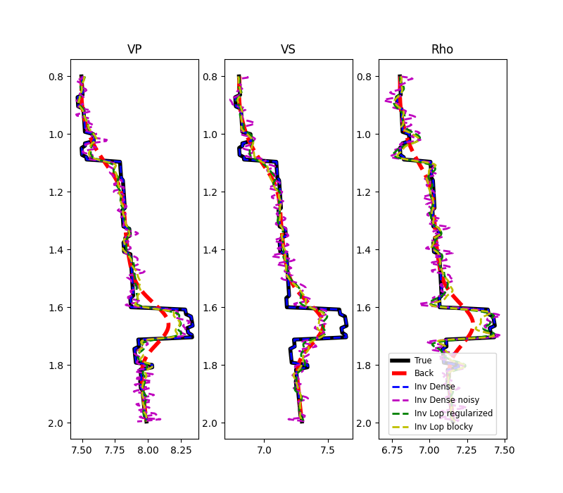
fig, axs = plt.subplots(1, 3, figsize=(8, 7))
for ip, param in enumerate(["VP", "VS", "Rho"]):
axs[ip].plot(m[:, ip, nx // 2], z, "k", lw=4, label="True")
axs[ip].plot(mback[:, ip, nx // 2], z, "--r", lw=4, label="Back")
axs[ip].plot(minv_dense[:, ip, nx // 2], z, "--b", lw=2, label="Inv Dense")
axs[ip].plot(
minv_dense_noisy[:, ip, nx // 2], z, "--m", lw=2, label="Inv Dense noisy"
)
axs[ip].plot(
minv_lop_reg[:, ip, nx // 2], z, "--g", lw=2, label="Inv Lop regularized"
)
axs[ip].plot(minv_blocky[:, ip, nx // 2], z, "--y", lw=2, label="Inv Lop blocky")
axs[ip].set_title(param)
axs[ip].invert_yaxis()
axs[2].legend(loc=8, fontsize="small")
Out:
<matplotlib.legend.Legend object at 0x7f4deb734080>
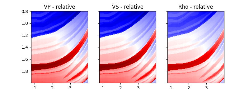
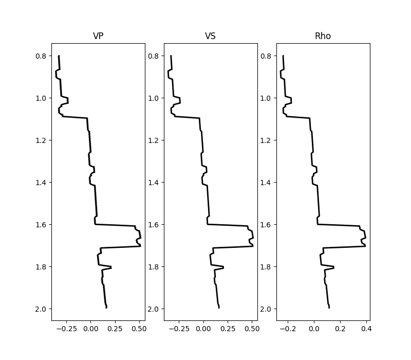
While the background model m0 has been provided in all the examples so
far, it is worth showing that the module
pylops.avo.prestack.PrestackInversion can also produce so-called
relative elastic parameters (i.e., variations from an average medium
property) when the background model m0 is not available.
dminv = pylops.avo.prestack.PrestackInversion(
    dPP, theta, wav, m0=None, explicit=True, simultaneous=False
)

fig, axs = plt.subplots(1, 3, figsize=(8, 3))
plotmodel(axs, dminv, x, z, -dminv.max(), dminv.max(), cmap="seismic", title="relative")

fig, axs = plt.subplots(1, 3, figsize=(8, 7))
for ip, param in enumerate(["VP", "VS", "Rho"]):
    axs[ip].plot(dminv[:, ip, nx // 2], z, "k", lw=2)
    axs[ip].set_title(param)
    axs[ip].invert_yaxis()
Total running time of the script: ( 1 minutes 0.351 seconds)