Note
Click here to download the full example code
03. Solvers
This tutorial will guide you through the pylops.optimization
module and show how to use various solvers that are included in the
PyLops library.
The main idea here is to provide the user of PyLops with very high-level functionalities to quickly and easily set up and solve complex systems of linear equations as well as include regularization and/or preconditioning terms (all of those constructed by means of PyLops linear operators).
To make this tutorial more interesting, we will present a real life problem and show how the choice of the solver and regularization/preconditioning terms is vital in many circumstances to successfully retrieve an estimate of the model. The problem that we are going to consider is generally referred to as the data reconstruction problem and aims at reconstructing a regularly sampled signal of size \(M\) from \(N\) randomly selected samples:
where the restriction operator \(\mathbf{R}\) that selects the \(M\)
elements from \(\mathbf{x}\) at random locations is implemented using
pylops.Restriction, and
with \(M \gg N\).
import matplotlib.pyplot as plt

# pylint: disable=C0103
import numpy as np

import pylops

plt.close("all")
np.random.seed(10)
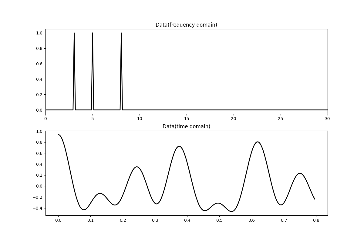
Let’s first create the data in the frequency domain. The data is composed by the superposition of 3 sinusoids with different frequencies.
# Signal creation in frequency domain
ifreqs = [41, 25, 66]
amps = [1.0, 1.0, 1.0]
N = 200
nfft = 2 ** 11
dt = 0.004
t = np.arange(N) * dt
f = np.fft.rfftfreq(nfft, dt)

FFTop = 10 * pylops.signalprocessing.FFT(N, nfft=nfft, real=True)

X = np.zeros(nfft // 2 + 1, dtype="complex128")
X[ifreqs] = amps
x = FFTop.H * X

fig, axs = plt.subplots(2, 1, figsize=(12, 8))
axs[0].plot(f, np.abs(X), "k", lw=2)
axs[0].set_xlim(0, 30)
axs[0].set_title("Data(frequency domain)")
axs[1].plot(t, x, "k", lw=2)
axs[1].set_title("Data(time domain)")
axs[1].axis("tight")
Out:
(-0.0398, 0.8358000000000001, -0.5341666861485157, 1.007579366007072)
We now define the locations at which the signal will be sampled.
# subsampling locations
perc_subsampling = 0.2
Nsub = int(np.round(N * perc_subsampling))

iava = np.sort(np.random.permutation(np.arange(N))[:Nsub])

# Create restriction operator
Rop = pylops.Restriction(N, iava, dtype="float64")

y = Rop * x
ymask = Rop.mask(x)

# Visualize data
fig = plt.figure(figsize=(12, 4))
plt.plot(t, x, "k", lw=3)
plt.plot(t, x, ".k", ms=20, label="all samples")
plt.plot(t, ymask, ".g", ms=15, label="available samples")
plt.legend()
plt.title("Data restriction")
Out:
Text(0.5, 1.0, 'Data restriction')
To start let’s consider the simplest ‘solver’, i.e., least-square inversion without regularization. We aim here to minimize the following cost function:
\[J = \|\mathbf{y} - \mathbf{R} \mathbf{x}\|_2^2\]
Depending on the choice of the operator \(\mathbf{R}\), such problem can
be solved using explicit matrix solvers as well as iterative solvers. In
this case we will be using the latter approach
(more specifically the scipy implementation of the LSQR solver -
i.e., scipy.sparse.linalg.lsqr) as we do not want to explicitly
create and invert a matrix. In most cases this will be the only viable
approach as most of the large-scale optimization problems that we are
interested to solve using PyLops do not lend naturally to the creation and
inversion of explicit matrices.
This first solver can be very easily implemented using the
/ for PyLops operators, which will automatically call the
scipy.sparse.linalg.lsqr with some default parameters.
We can also use pylops.optimization.leastsquares.RegularizedInversion
(without regularization term for now) and customize our solvers using
kwargs.
xinv = pylops.optimization.leastsquares.RegularizedInversion(
    Rop, [], y, **dict(damp=0, iter_lim=10, show=1)
)
Out:
LSQR            Least-squares solution of  Ax = b
The matrix A has 40 rows and 200 columns
damp = 0.00000000000000e+00   calc_var =        0
atol = 1.00e-08                 conlim = 1.00e+08
btol = 1.00e-08               iter_lim =       10

   Itn      x[0]       r1norm     r2norm   Compatible    LS      Norm A   Cond A
     0  0.00000e+00   2.658e+00  2.658e+00    1.0e+00  3.8e-01
     1  0.00000e+00   0.000e+00  0.000e+00    0.0e+00  0.0e+00   0.0e+00  0.0e+00

LSQR finished
Ax - b is small enough, given atol, btol

istop =       1   r1norm = 0.0e+00   anorm = 0.0e+00   arnorm = 0.0e+00
itn   =       1   r2norm = 0.0e+00   acond = 0.0e+00   xnorm  = 2.7e+00
Finally we can select a different starting guess from the null vector
xinv_fromx0 = pylops.optimization.leastsquares.RegularizedInversion(
    Rop, [], y, x0=np.ones(N), **dict(damp=0, iter_lim=10, show=0)
)
The cost function above can be also expanded in terms of its normal equations
\[\mathbf{x}_{ne}= (\mathbf{R}^T \mathbf{R})^{-1} \mathbf{R}^T \mathbf{y}\]
The method pylops.optimization.leastsquares.NormalEquationsInversion
implements such system of equations explicitly and solves them using an
iterative scheme suitable for square matrices (i.e., \(M=N\)).
While this approach may seem not very useful, we will soon see how regularization terms could be easily added to the normal equations using this method.
Let’s now visualize the different inversion results
fig = plt.figure(figsize=(12, 4))
plt.plot(t, x, "k", lw=2, label="original")
plt.plot(t, xinv, "b", ms=10, label="inversion")
plt.plot(t, xinv_fromx0, "--r", ms=10, label="inversion from x0")
plt.plot(t, xne, "--g", ms=10, label="normal equations")
plt.legend()
plt.title("Data reconstruction without regularization")
Out:
Text(0.5, 1.0, 'Data reconstruction without regularization')
Regularization
You may have noticed that none of the inversion has been successfull in recovering the original signal. This is a clear indication that the problem we are trying to solve is highly ill-posed and requires some prior knowledge from the user.
We will now see how to add prior information to the inverse process in the form of regularization (or preconditioning). This can be done in two different ways
- regularization via
pylops.optimization.leastsquares.NormalEquationsInversionorpylops.optimization.leastsquares.RegularizedInversion) - preconditioning via
pylops.optimization.leastsquares.PreconditionedInversion
Let’s start by regularizing the normal equations using a second derivative operator
\[\mathbf{x} = (\mathbf{R^TR}+\epsilon_\nabla^2\nabla^T\nabla)^{-1} \mathbf{R^Ty}\]
# Create regularization operator
D2op = pylops.SecondDerivative(N, dims=None, dtype="float64")

# Regularized inversion
epsR = np.sqrt(0.1)
epsI = np.sqrt(1e-4)

xne = pylops.optimization.leastsquares.NormalEquationsInversion(
    Rop, [D2op], y, epsI=epsI, epsRs=[epsR], returninfo=False, **dict(maxiter=50)
)
Note that in case we have access to a fast implementation for the chain of
forward and adjoint for the regularization operator
(i.e., \(\nabla^T\nabla\)), we can modify our call to
pylops.optimization.leastsquares.NormalEquationsInversion as
follows:
We can do the same while using
pylops.optimization.leastsquares.RegularizedInversion
which solves the following augmented problem
\[\begin{split}\begin{bmatrix} \mathbf{R} \\ \epsilon_\nabla \nabla \end{bmatrix} \mathbf{x} = \begin{bmatrix} \mathbf{y} \\ 0 \end{bmatrix}\end{split}\]
We can also write a preconditioned problem, whose cost function is
\[J= \|\mathbf{y} - \mathbf{R} \mathbf{P} \mathbf{p}\|_2^2\]
where \(\mathbf{P}\) is the precondioned operator, \(\mathbf{p}\) is
the projected model in the preconditioned space, and
\(\mathbf{x}=\mathbf{P}\mathbf{p}\) is the model in the original model
space we want to solve for. Note that a preconditioned problem converges
much faster to its solution than its corresponding regularized problem.
This can be done using the routine
pylops.optimization.leastsquares.PreconditionedInversion.
# Create regularization operator
Sop = pylops.Smoothing1D(nsmooth=11, dims=[N], dtype="float64")

# Invert for interpolated signal
xprec = pylops.optimization.leastsquares.PreconditionedInversion(
    Rop, Sop, y, returninfo=False, **dict(damp=np.sqrt(1e-9), iter_lim=20, show=0)
)
Let’s finally visualize these solutions
# sphinx_gallery_thumbnail_number=4
fig = plt.figure(figsize=(12, 4))
plt.plot(t[iava], y, ".k", ms=20, label="available samples")
plt.plot(t, x, "k", lw=3, label="original")
plt.plot(t, xne, "b", lw=3, label="normal equations")
plt.plot(t, xne1, "--c", lw=3, label="normal equations (with direct D^T D)")
plt.plot(t, xreg, "-.r", lw=3, label="regularized")
plt.plot(t, xprec, "--g", lw=3, label="preconditioned equations")
plt.legend()
plt.title("Data reconstruction with regularization")

subax = fig.add_axes([0.7, 0.2, 0.15, 0.6])
subax.plot(t[iava], y, ".k", ms=20)
subax.plot(t, x, "k", lw=3)
subax.plot(t, xne, "b", lw=3)
subax.plot(t, xne1, "--c", lw=3)
subax.plot(t, xreg, "-.r", lw=3)
subax.plot(t, xprec, "--g", lw=3)
subax.set_xlim(0.05, 0.3)
Out:
(0.05, 0.3)
Much better estimates! We have seen here how regularization and/or preconditioning can be vital to succesfully solve some ill-posed inverse problems.
We have however so far only considered solvers that can include additional norm-2 regularization terms. A very active area of research is that of sparsity-promoting solvers (also sometimes referred to as compressive sensing): the regularization term added to the cost function to minimize has norm-p (\(p \le 1\)) and the problem is generally recasted by considering the model to be sparse in some domain. We can follow this philosophy as our signal to invert was actually created as superposition of 3 sinusoids (i.e., three spikes in the Fourier domain). Our new cost function is:
\[J_1 = \|\mathbf{y} - \mathbf{R} \mathbf{F} \mathbf{p}\|_2^2 + \epsilon \|\mathbf{p}\|_1\]
where \(\mathbf{F}\) is the FFT operator. We will thus use the
pylops.optimization.sparsity.ISTA and
pylops.optimization.sparsity.FISTA solvers to estimate our input
signal.
pista, niteri, costi = pylops.optimization.sparsity.ISTA(
    Rop * FFTop.H, y, niter=1000, eps=0.1, tol=1e-7, returninfo=True
)
xista = FFTop.H * pista

pfista, niterf, costf = pylops.optimization.sparsity.FISTA(
    Rop * FFTop.H, y, niter=1000, eps=0.1, tol=1e-7, returninfo=True
)
xfista = FFTop.H * pfista

fig, axs = plt.subplots(2, 1, figsize=(12, 8))
fig.suptitle("Data reconstruction with sparsity", fontsize=14, fontweight="bold", y=0.9)
axs[0].plot(f, np.abs(X), "k", lw=3)
axs[0].plot(f, np.abs(pista), "--r", lw=3)
axs[0].plot(f, np.abs(pfista), "--g", lw=3)
axs[0].set_xlim(0, 30)
axs[0].set_title("Frequency domain")
axs[1].plot(t[iava], y, ".k", ms=20, label="available samples")
axs[1].plot(t, x, "k", lw=3, label="original")
axs[1].plot(t, xista, "--r", lw=3, label="ISTA")
axs[1].plot(t, xfista, "--g", lw=3, label="FISTA")
axs[1].set_title("Time domain")
axs[1].axis("tight")
axs[1].legend()
plt.tight_layout()
plt.subplots_adjust(top=0.8)

fig, ax = plt.subplots(1, 1, figsize=(12, 3))
ax.semilogy(costi, "r", lw=2, label="ISTA")
ax.semilogy(costf, "g", lw=2, label="FISTA")
ax.set_title("Cost functions", size=15, fontweight="bold")
ax.set_xlabel("Iteration")
ax.legend()
ax.grid(True)
plt.tight_layout()
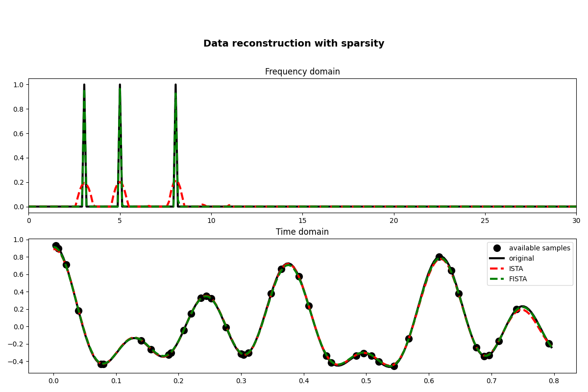
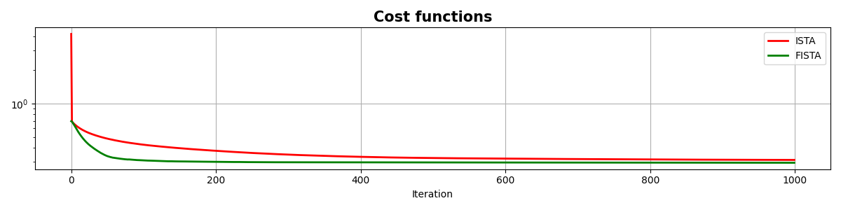
As you can see, changing parametrization of the model and imposing sparsity in the Fourier domain has given an extra improvement to our ability of recovering the underlying densely sampled input signal. Moreover, FISTA converges much faster than ISTA as expected and should be preferred when using sparse solvers.
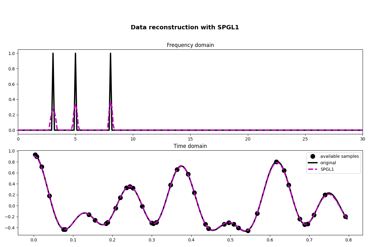
Finally we consider a slightly different cost function (note that in this case we try to solve a constrained problem):
\[J_1 = \|\mathbf{p}\|_1 \quad \text{subject to} \quad \|\mathbf{y} - \mathbf{R} \mathbf{F} \mathbf{p}\|\]
A very popular solver to solve such kind of cost function is called spgl1
and can be accessed via pylops.optimization.sparsity.SPGL1.
xspgl1, pspgl1, info = pylops.optimization.sparsity.SPGL1(
Rop, y, FFTop, tau=3, iter_lim=200
)
fig, axs = plt.subplots(2, 1, figsize=(12, 8))
fig.suptitle("Data reconstruction with SPGL1", fontsize=14, fontweight="bold", y=0.9)
axs[0].plot(f, np.abs(X), "k", lw=3)
axs[0].plot(f, np.abs(pspgl1), "--m", lw=3)
axs[0].set_xlim(0, 30)
axs[0].set_title("Frequency domain")
axs[1].plot(t[iava], y, ".k", ms=20, label="available samples")
axs[1].plot(t, x, "k", lw=3, label="original")
axs[1].plot(t, xspgl1, "--m", lw=3, label="SPGL1")
axs[1].set_title("Time domain")
axs[1].axis("tight")
axs[1].legend()
plt.tight_layout()
plt.subplots_adjust(top=0.8)
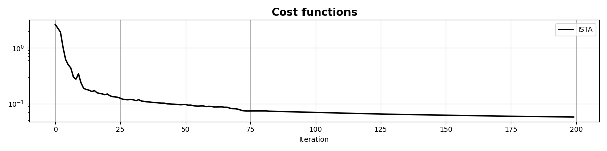
fig, ax = plt.subplots(1, 1, figsize=(12, 3))
ax.semilogy(info["rnorm2"], "k", lw=2, label="ISTA")
ax.set_title("Cost functions", size=15, fontweight="bold")
ax.set_xlabel("Iteration")
ax.legend()
ax.grid(True)
plt.tight_layout()
Total running time of the script: ( 0 minutes 6.622 seconds)