pylops.optimization.solver.lsqr
-
pylops.optimization.solver.lsqr(Op, y, x0, damp=0.0, atol=1e-08, btol=1e-08, conlim=100000000.0, niter=10, calc_var=True, show=False, callback=None)[source]¶ LSQR
Solve an overdetermined system of equations given an operator
Opand datayusing LSQR iterations.\[\DeclareMathOperator{\cond}{cond}\]Parameters: - Op :
pylops.LinearOperator Operator to invert of size \([N \times M]\)
- y :
np.ndarray Data of size \([N \times 1]\)
- x0 :
np.ndarray, optional Initial guess
- damp :
float, optional Damping coefficient
- atol, btol :
float, optional Stopping tolerances. If both are 1.0e-9, the final residual norm should be accurate to about 9 digits. (The solution will usually have fewer correct digits, depending on \(\cond(\mathbf{Op})\) and the size of
damp.)- conlim :
float, optional Stopping tolerance on \(\cond(\mathbf{Op})\) exceeds
conlim. For square,conlimcould be as large as 1.0e+12. For least-squares problems,conlimshould be less than 1.0e+8. Maximum precision can be obtained by settingatol = btol = conlim = 0, but the number of iterations may then be excessive.- niter :
int, optional Number of iterations
- calc_var :
bool, optional Estimate diagonals of \((\mathbf{Op}^H\mathbf{Op} + \epsilon^2\mathbf{I})^{-1}\).
- show :
bool, optional Display iterations log
- callback :
callable, optional Function with signature (
callback(x)) to call after each iteration wherexis the current model vector
Returns: - x :
np.ndarray Estimated model of size \([M \times 1]\)
- istop :
int Gives the reason for termination
0means the exact solution is \(\mathbf{x}=0\)1means \(\mathbf{x}\) is an approximate solution to \(\mathbf{y} = \mathbf{Op}\,\mathbf{x}\)2means \(\mathbf{x}\) approximately solves the least-squares problem3means the estimate of \(\cond(\overline{\mathbf{Op}})\) has exceededconlim4means \(\mathbf{y} - \mathbf{Op}\,\mathbf{x}\) is small enough for this machine5means the least-squares solution is good enough for this machine6means \(\cond(\overline{\mathbf{Op}})\) seems to be too large for this machine7means the iteration limit has been reached- r1norm :
float \(||\mathbf{r}||_2^2\), where \(\mathbf{r} = \mathbf{y} - \mathbf{Op}\,\mathbf{x}\)
- r2norm :
float \(\sqrt{\mathbf{r}^T\mathbf{r} + \epsilon^2 \mathbf{x}^T\mathbf{x}}\). Equal to
r1normif \(\epsilon=0\)- anorm :
float Estimate of Frobenius norm of \(\overline{\mathbf{Op}} = [\mathbf{Op} \; \epsilon \mathbf{I}]\)
- acond :
float Estimate of \(\cond(\overline{\mathbf{Op}})\)
- arnorm :
float Estimate of norm of \(\cond(\mathbf{Op}^H\mathbf{r}- \epsilon^2\mathbf{x})\)
- var :
float Diagonals of \((\mathbf{Op}^H\mathbf{Op})^{-1}\) (if
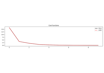
damp=0) or more generally \((\mathbf{Op}^H\mathbf{Op} + \epsilon^2\mathbf{I})^{-1}\).- cost :
numpy.ndarray, optional History of r1norm through iterations
Notes
Minimize the following functional using LSQR iterations [1]:
\[J = || \mathbf{y} - \mathbf{Op}\,\mathbf{x} ||_2^2 + \epsilon^2 || \mathbf{x} ||_2^2\]where \(\epsilon\) is the damping coefficient.
[1] Paige, C. C., and Saunders, M. A. “LSQR: An algorithm for sparse linear equations and sparse least squares”, ACM TOMS, vol. 8, pp. 43-71, 1982. - Op :
