Total Variation (TV) Regularization

This set of examples shows how to add Total Variation (TV) regularization to an inverse problem in order to enforce blockiness in the reconstructed model.

To do so we will use the generalizated Split Bregman iterations by means of pylops.optimization.sparsity.SplitBregman solver.

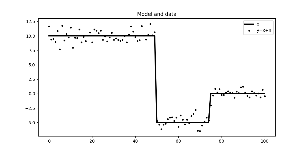
The first example is concerned with denoising of a piece-wise step function which has been contaminated by noise. The forward model is:

\[\mathbf{y} = \mathbf{x} + \mathbf{n}\]

meaning that we have an identity operator (\(\mathbf{I}\)) and inverting for \(\mathbf{x}\) from \(\mathbf{y}\) is impossible without adding prior information. We will enforce blockiness in the solution by adding a regularization term that enforces sparsity in the first derivative of the solution:

\[J = \mu/2 ||\mathbf{y} - \mathbf{I} \mathbf{x}||_2 + || \nabla \mathbf{x}||_1\]

# sphinx_gallery_thumbnail_number = 5
import numpy as np
import matplotlib.pyplot as plt

import pylops

plt.close('all')
np.random.seed(1)

Let’s start by creating the model and data

nx = 101
x = np.zeros(nx)
x[:nx//2] = 10
x[nx//2:3*nx//4] = -5

Iop = pylops.Identity(nx)

n = np.random.normal(0, 1, nx)
y = Iop*(x + n)

plt.figure(figsize=(10, 5))
plt.plot(x, 'k', lw=3, label='x')
plt.plot(y, '.k', label='y=x+n')
plt.legend()
plt.title('Model and data')

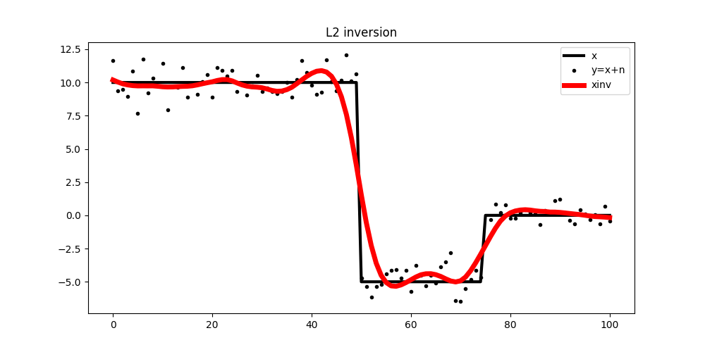
To start we will try to use a simple L2 regularization that enforces smoothness in the solution. We can see how denoising is succesfully achieved but the solution is much smoother than we wish for.

D2op = pylops.SecondDerivative(nx, edge=True)
lamda = 1e2

xinv = \
    pylops.optimization.leastsquares.RegularizedInversion(Iop, [D2op], y,
                                                          epsRs=[np.sqrt(lamda/2)],
                                                          **dict(iter_lim=30))

plt.figure(figsize=(10, 5))
plt.plot(x, 'k', lw=3, label='x')
plt.plot(y, '.k', label='y=x+n')
plt.plot(xinv, 'r', lw=5, label='xinv')
plt.legend()
plt.title('L2 inversion')

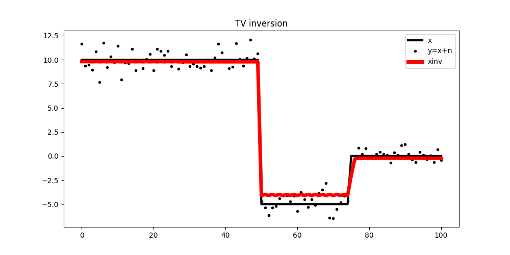
Now we impose blockiness in the solution using the Split Bregman solver

Dop = pylops.FirstDerivative(nx, edge=True)
mu = 0.01
lamda = 0.3
niter_out = 50
niter_in = 3

xinv, niter = \
    pylops.optimization.sparsity.SplitBregman(Iop, [Dop], y, niter_out,
                                              niter_in, mu=mu, epsRL1s=[lamda],
                                              tol=1e-4, tau=1.,
                                              **dict(iter_lim=30, damp=1e-10))

plt.figure(figsize=(10, 5))
plt.plot(x, 'k', lw=3, label='x')
plt.plot(y, '.k', label='y=x+n')
plt.plot(xinv, 'r', lw=5, label='xinv')
plt.legend()
plt.title('TV inversion')

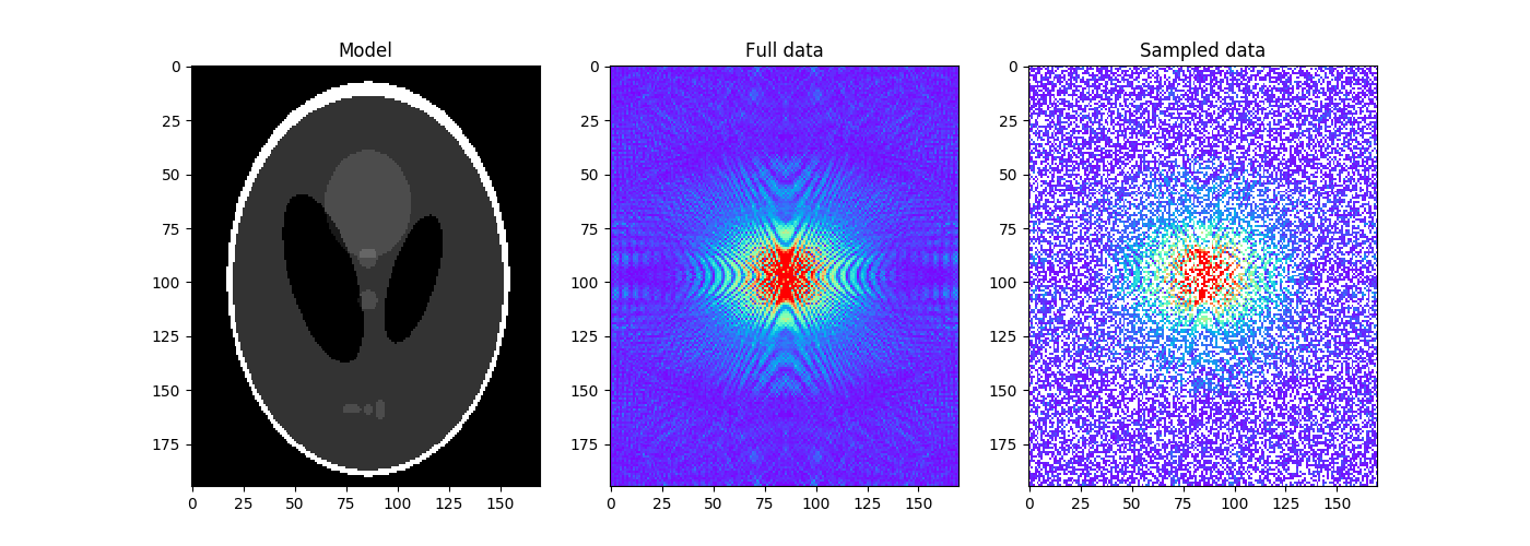
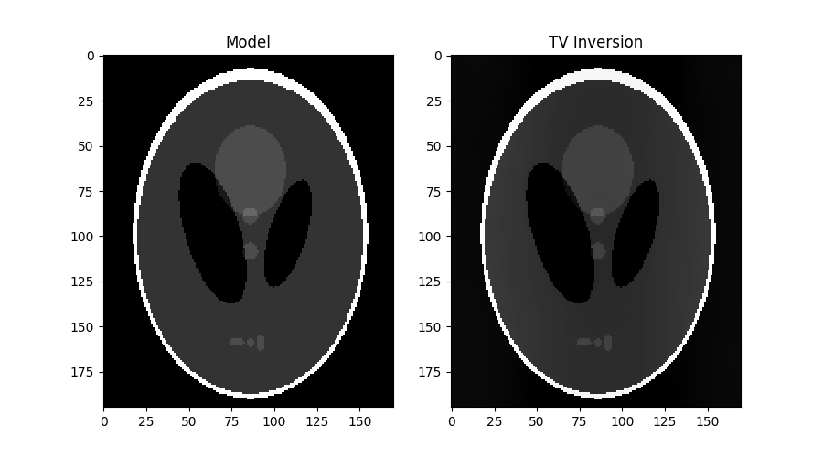
Finally, we repeat the same exercise on a 2-dimensional image. In this case we however consider the MRI imaging problem where the Split Bregman solver shines. The data is created by first appling a 2D Fourier Transform of the input model and by randomly sampling 60% of its values.

x = np.load('../testdata/optimization/shepp_logan_phantom.npy')
x = x/x.max()
ny, nx = x.shape

perc_subsampling = 0.6
nxsub = int(np.round(ny*nx*perc_subsampling))
iava = np.sort(np.random.permutation(np.arange(ny*nx))[:nxsub])
Rop = pylops.Restriction(ny*nx, iava, dtype=np.complex)
Fop = pylops.signalprocessing.FFT2D(dims=(ny, nx))

n = np.random.normal(0, 0., (ny, nx))
y = Rop*Fop*(x.flatten() + n.flatten())
yfft = Fop*(x.flatten() + n.flatten())
yfft = np.fft.fftshift(yfft.reshape(ny, nx))

ymask = Rop.mask(Fop*(x.flatten()) + n.flatten())
ymask = ymask.reshape(ny, nx)
ymask.data[:] = np.fft.fftshift(ymask.data)
ymask.mask[:] = np.fft.fftshift(ymask.mask)

fig, axs = plt.subplots(1, 3, figsize=(14, 5))
axs[0].imshow(x, vmin=0, vmax=1, cmap='gray')
axs[0].set_title('Model')
axs[0].axis('tight')
axs[1].imshow(np.abs(yfft), vmin=0, vmax=1, cmap='rainbow')
axs[1].set_title('Full data')
axs[1].axis('tight')
axs[2].imshow(np.abs(ymask), vmin=0, vmax=1, cmap='rainbow')
axs[2].set_title('Sampled data')
axs[2].axis('tight')

Let’s attempt now to reconstruct the model using the Split Bregman with anisotropic TV regularization (aka sum of L1 norms of the first derivatives over x and y):

\[J = \mu/2 ||\mathbf{y} - \mathbf{R} \mathbf{F} \mathbf{x}||_2 + || \nabla_x \mathbf{x}||_1 + || \nabla_y \mathbf{x}||_1\]

#Dop = \
#    [pylops.FirstDerivative(ny * nx, dims=(ny, nx), dir=0, edge=False, dtype=np.complex) + \
#     pylops.FirstDerivative(ny * nx, dims=(ny, nx), dir=1, edge=False, dtype=np.complex)]
Dop = \
    [pylops.FirstDerivative(ny * nx, dims=(ny, nx), dir=0, edge=False, dtype=np.complex),
     pylops.FirstDerivative(ny * nx, dims=(ny, nx), dir=1, edge=False, dtype=np.complex)]

# TV
mu = 1.5
lamda = [0.1, 0.1]
niter = 20
niterinner = 10

xinv, niter = \
    pylops.optimization.sparsity.SplitBregman(Rop * Fop, Dop, y.flatten(),
                                              niter, niterinner,
                                              mu=mu, epsRL1s=lamda,
                                              tol=1e-4, tau=1., show=False,
                                              **dict(iter_lim=5, damp=1e-4))
xinv = np.real(xinv.reshape(ny, nx))

fig, axs = plt.subplots(1, 2, figsize=(9, 5))
axs[0].imshow(x, vmin=0, vmax=1, cmap='gray')
axs[0].set_title('Model')
axs[0].axis('tight')
axs[1].imshow(xinv, vmin=0, vmax=1, cmap='gray')
axs[1].set_title('TV Inversion')
axs[1].axis('tight')

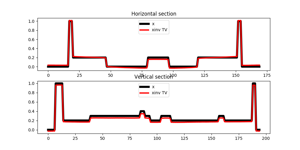
fig, axs = plt.subplots(2, 1, figsize=(10, 5))
axs[0].plot(x[ny//2], 'k', lw=5, label='x')
axs[0].plot(xinv[ny//2], 'r', lw=3, label='xinv TV')
axs[0].set_title('Horizontal section')
axs[0].legend()
axs[1].plot(x[:, nx//2], 'k', lw=5, label='x')
axs[1].plot(xinv[:, nx//2], 'r', lw=3, label='xinv TV')
axs[1].set_title('Vertical section')
axs[1].legend()

• 
• 

Note that more optimized variations of the Split Bregman algorithm have been proposed in the literature for this specific problem, both improving the overall quality of the inversion and the speed of convergence.

In PyLops we however prefer to implement the generalized Split Bergman algorithm as this can used for any sort of problem where we wish to add any number of L1 and/or L2 regularization terms to the cost function to minimize.