Note
Click here to download the full example code
04. Bayesian Inversion
This tutorial focuses on Bayesian inversion, a special type of inverse problem that aims at incorporating prior information in terms of model and data probabilities in the inversion process.
In this case we will be dealing with the same problem that we discussed in 03. Solvers, but instead of defining ad-hoc regularization or preconditioning terms we parametrize and model our input signal in the frequency domain in a probabilistic fashion: the central frequency, amplitude and phase of the three sinusoids have gaussian distributions as follows:
where \(f_i \sim N(f_{0,i}, \sigma_{f,i})\), \(a_i \sim N(a_{0,i}, \sigma_{a,i})\), and \(\phi_i \sim N(\phi_{0,i}, \sigma_{\phi,i})\).
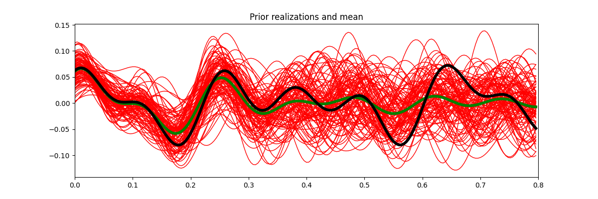
Based on the above definition, we construct some prior models in the frequency domain, convert each of them to the time domain and use such an ensemble to estimate the prior mean \(\mu_\mathbf{x}\) and model covariance \(\mathbf{C_x}\).
We then create our data by sampling the true signal at certain locations and solve the resconstruction problem within a Bayesian framework. Since we are assuming gaussianity in our priors, the equation to obtain the posterion mean can be derived analytically:
import matplotlib.pyplot as plt

# sphinx_gallery_thumbnail_number = 2
import numpy as np
from scipy.sparse.linalg import lsqr

import pylops

plt.close("all")
np.random.seed(10)
Let’s start by creating our true model and prior realizations
def prior_realization(f0, a0, phi0, sigmaf, sigmaa, sigmaphi, dt, nt, nfft):
    """Create realization from prior mean and std for amplitude, frequency and
    phase
    """
    f = np.fft.rfftfreq(nfft, dt)
    df = f[1] - f[0]
    ifreqs = [int(np.random.normal(f, sigma) / df) for f, sigma in zip(f0, sigmaf)]
    amps = [np.random.normal(a, sigma) for a, sigma in zip(a0, sigmaa)]
    phis = [np.random.normal(phi, sigma) for phi, sigma in zip(phi0, sigmaphi)]

    # input signal in frequency domain
    X = np.zeros(nfft // 2 + 1, dtype="complex128")
    X[ifreqs] = (
        np.array(amps).squeeze() * np.exp(1j * np.deg2rad(np.array(phis))).squeeze()
    )

    # input signal in time domain
    FFTop = pylops.signalprocessing.FFT(nt, nfft=nfft, real=True)
    x = FFTop.H * X
    return x


# Priors
nreals = 100
f0 = [5, 3, 8]
sigmaf = [0.5, 1.0, 0.6]
a0 = [1.0, 1.0, 1.0]
sigmaa = [0.1, 0.5, 0.6]
phi0 = [-90.0, 0.0, 0.0]
sigmaphi = [0.1, 0.2, 0.4]
sigmad = 1e-2

# Prior models
nt = 200
nfft = 2**11
dt = 0.004
t = np.arange(nt) * dt
xs = np.array(
    [
        prior_realization(f0, a0, phi0, sigmaf, sigmaa, sigmaphi, dt, nt, nfft)
        for _ in range(nreals)
    ]
)

# True model (taken as one possible realization)
x = prior_realization(f0, a0, phi0, [0, 0, 0], [0, 0, 0], [0, 0, 0], dt, nt, nfft)
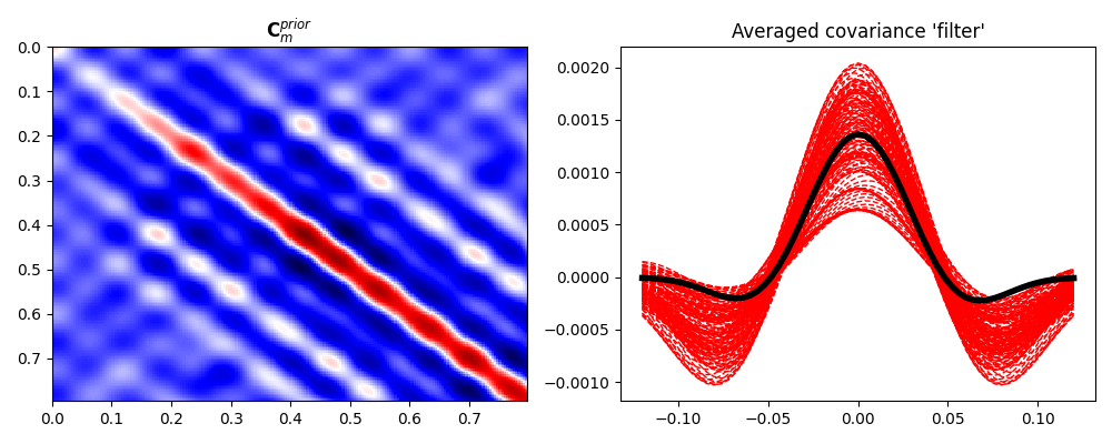
We have now a set of prior models in time domain. We can easily use sample statistics to estimate the prior mean and covariance. For the covariance, we perform a second step where we average values around the main diagonal for each row and find a smooth, compact filter that we use to define a convolution linear operator that mimics the action of the covariance matrix on a vector
x0 = np.average(xs, axis=0)
Cm = ((xs - x0).T @ (xs - x0)) / nreals

N = 30  # lenght of decorrelation
diags = np.array([Cm[i, i - N : i + N + 1] for i in range(N, nt - N)])
diag_ave = np.average(diags, axis=0)
# add a taper at the end to avoid edge effects
diag_ave *= np.hamming(2 * N + 1)

fig, ax = plt.subplots(1, 1, figsize=(12, 4))
ax.plot(t, xs.T, "r", lw=1)
ax.plot(t, x0, "g", lw=4)
ax.plot(t, x, "k", lw=4)
ax.set_title("Prior realizations and mean")
ax.set_xlim(0, 0.8)

fig, (ax1, ax2) = plt.subplots(1, 2, figsize=(10, 4))
im = ax1.imshow(
    Cm, interpolation="nearest", cmap="seismic", extent=(t[0], t[-1], t[-1], t[0])
)
ax1.set_title(r"$\mathbf{C}_m^{prior}$")
ax1.axis("tight")
ax2.plot(np.arange(-N, N + 1) * dt, diags.T, "--r", lw=1)
ax2.plot(np.arange(-N, N + 1) * dt, diag_ave, "k", lw=4)
ax2.set_title("Averaged covariance 'filter'")
plt.tight_layout()
Let’s define now the sampling operator as well as create our covariance matrices in terms of linear operators. This may not be strictly necessary here but shows how even Bayesian-type of inversion can very easily scale to large model and data spaces.
# Sampling operator
perc_subsampling = 0.2
ntsub = int(np.round(nt * perc_subsampling))
iava = np.sort(np.random.permutation(np.arange(nt))[:ntsub])
iava[-1] = nt - 1  # assume we have the last sample to avoid instability
Rop = pylops.Restriction(nt, iava, dtype="float64")

# Covariance operators
Cm_op = pylops.signalprocessing.Convolve1D(nt, diag_ave, offset=N)
Cd_op = sigmad**2 * pylops.Identity(ntsub)
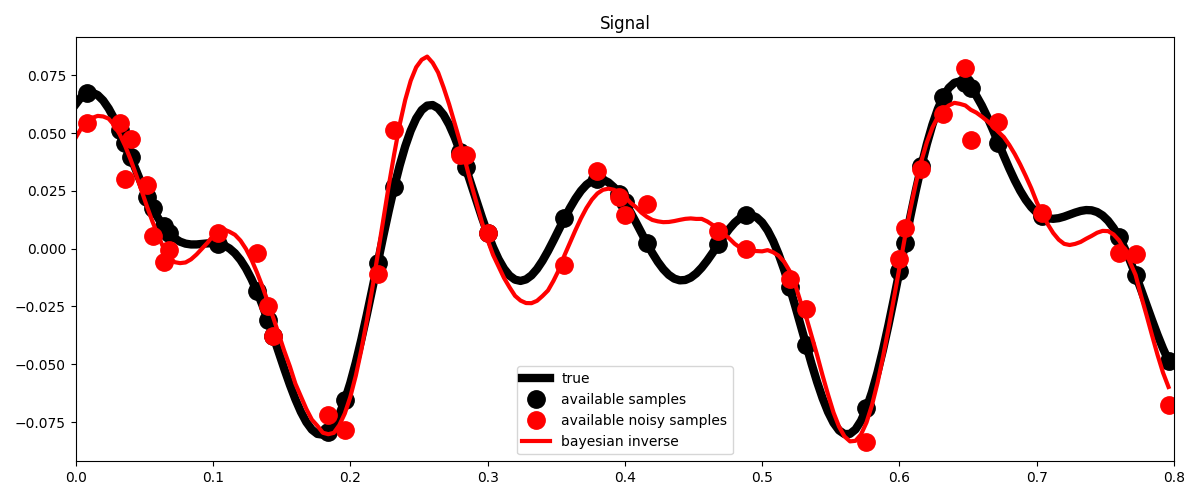
We model now our data and add noise that respects our prior definition
First we apply the Bayesian inversion equation
xbayes = x0 + Cm_op * Rop.H * (
    lsqr(Rop * Cm_op * Rop.H + Cd_op, yn - Rop * x0, iter_lim=400)[0]
)

# Visualize
fig, ax = plt.subplots(1, 1, figsize=(12, 5))
ax.plot(t, x, "k", lw=6, label="true")
ax.plot(t, ymask, ".k", ms=25, label="available samples")
ax.plot(t, ynmask, ".r", ms=25, label="available noisy samples")
ax.plot(t, xbayes, "r", lw=3, label="bayesian inverse")
ax.legend()
ax.set_title("Signal")
ax.set_xlim(0, 0.8)
plt.tight_layout()
So far we have been able to estimate our posterion mean. What about its uncertainties (i.e., posterion covariance)?
In real-life applications it is very difficult (if not impossible) to directly compute the posterior covariance matrix. It is much more useful to create a set of models that sample the posterion probability. We can do that by solving our problem several times using different prior realizations as starting guesses:
xpost = [
    x0
    + Cm_op
    * Rop.H
    * (lsqr(Rop * Cm_op * Rop.H + Cd_op, yn - Rop * x0, iter_lim=400)[0])
    for x0 in xs[:30]
]
xpost = np.array(xpost)

x0post = np.average(xpost, axis=0)
Cm_post = ((xpost - x0post).T @ (xpost - x0post)) / nreals

# Visualize
fig, ax = plt.subplots(1, 1, figsize=(12, 5))
ax.plot(t, x, "k", lw=6, label="true")
ax.plot(t, xpost.T, "--r", lw=1)
ax.plot(t, x0post, "r", lw=3, label="bayesian inverse")
ax.plot(t, ymask, ".k", ms=25, label="available samples")
ax.plot(t, ynmask, ".r", ms=25, label="available noisy samples")
ax.legend()
ax.set_title("Signal")
ax.set_xlim(0, 0.8)

fig, ax = plt.subplots(1, 1, figsize=(5, 4))
im = ax.imshow(
    Cm_post, interpolation="nearest", cmap="seismic", extent=(t[0], t[-1], t[-1], t[0])
)
ax.set_title(r"$\mathbf{C}_m^{posterior}$")
ax.axis("tight")
plt.tight_layout()
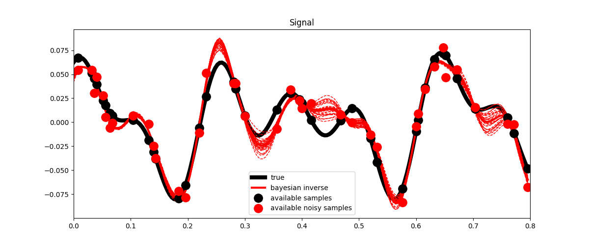
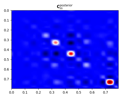
Note that here we have been able to compute a sample posterior covariance from its estimated samples. By displaying it we can see how both the overall variances and the correlation between different parameters have become narrower compared to their prior counterparts.
Total running time of the script: ( 0 minutes 1.659 seconds)