Note
Click here to download the full example code
03. Solvers (Advanced)
This is a follow up tutorial to the 03. Solvers tutorial. The same example will be considered, however we will showcase how to use the class-based version of our solvers (introduced in PyLops v2).
First of all, when shall you use class-based solvers over function-based ones? The answer is simple, every time you feel you would have like to have more flexibility when using one PyLops function-based solvers.
In fact, a function-based solver in PyLops v2 is nothing more than a thin wrapper over its class-based equivalent, which generally performs the following steps:
solver initialization
setuprun(by calling multiple timesstep)finalize
The nice thing about class-based solvers is that i) a user can manually orchestrate these steps and do anything
in between them; ii) a user can create a class-based pylops.optimization.callback.Callbacks object and
define a set of callbacks that will be run pre and post setup, step and run. One example of how such callbacks can
be handy to track evolving variables in the solver can be found in Linear Regression.
In the following we will leverage the very same mechanism to keep track of a number of metrics using the predefined
pylops.optimization.callback.MetricsCallback callback. Finally we show how to create a customized callback
that can track the percentage change of the solution and residual. This is of course just an example, we expect
users will find different use cases based on the problem at hand.
import matplotlib.pyplot as plt

# pylint: disable=C0103
import numpy as np

import pylops

plt.close("all")
np.random.seed(10)
Let’s first create the data in the frequency domain. The data is composed by the superposition of 3 sinusoids with different frequencies.
# Signal creation in frequency domain
ifreqs = [41, 25, 66]
amps = [1.0, 1.0, 1.0]
N = 200
nfft = 2**11
dt = 0.004
t = np.arange(N) * dt
f = np.fft.rfftfreq(nfft, dt)

FFTop = 10 * pylops.signalprocessing.FFT(N, nfft=nfft, real=True)

X = np.zeros(nfft // 2 + 1, dtype="complex128")
X[ifreqs] = amps
x = FFTop.H * X
We now define the locations at which the signal will be sampled.
# subsampling locations
perc_subsampling = 0.2
Nsub = int(np.round(N * perc_subsampling))

iava = np.sort(np.random.permutation(np.arange(N))[:Nsub])

# Create restriction operator
Rop = pylops.Restriction(N, iava, dtype="float64")

y = Rop * x
ymask = Rop.mask(x)
Let’s now solve the interpolation problem using the
pylops.optimization.sparsity.ISTA class-based solver.
cb = pylops.optimization.callback.MetricsCallback(x, FFTop.H)
istasolve = pylops.optimization.sparsity.ISTA(
Rop * FFTop.H,
callbacks=[
cb,
],
)
pista, niteri, costi = istasolve.solve(y, niter=1000, eps=0.1, tol=1e-7)
xista = FFTop.H * pista
fig, axs = plt.subplots(1, 4, figsize=(16, 3))
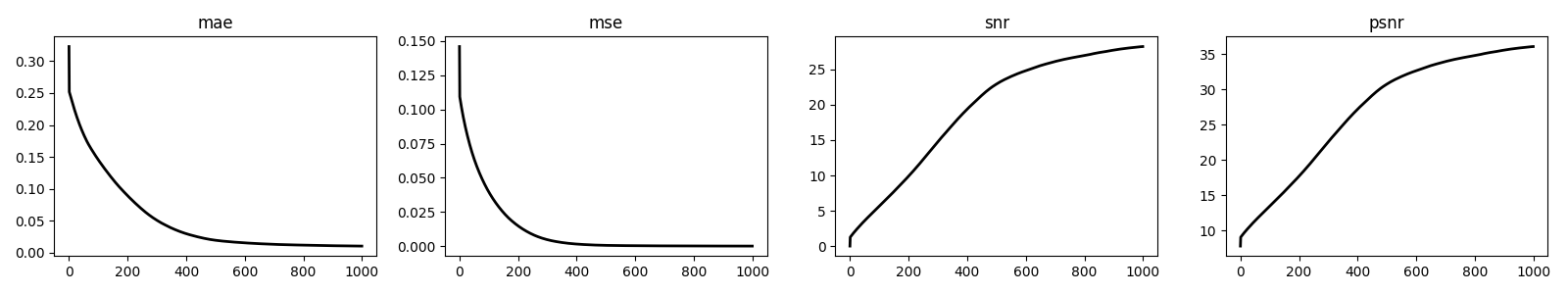
for i, metric in enumerate(["mae", "mse", "snr", "psnr"]):
axs[i].plot(cb.metrics[metric], "k", lw=2)
axs[i].set_title(metric)
plt.tight_layout()
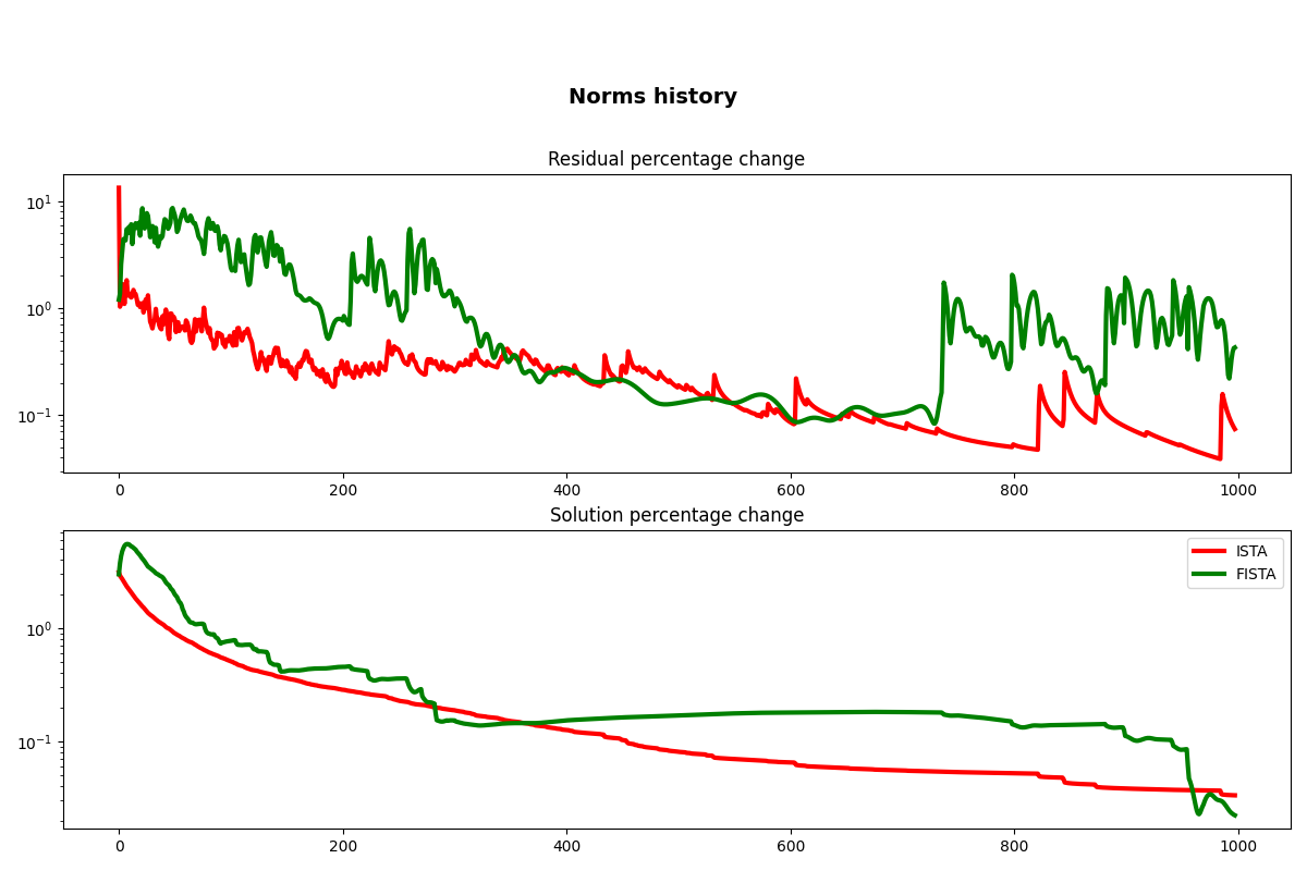
Finally, we show how we can also define customized callbacks. What we are really interested in here is to store the first residual norm once the setup of the solver is over, and repeat the same after each step (using the previous estimate to compute the percentage change). And, we do the same for the solution norm.
class CallbackISTA(pylops.optimization.callback.Callbacks):
def __init__(self):
self.res_perc = []
self.x_perc = []
def on_setup_end(self, solver, x):
self.x = x
if x is not None:
self.rec = solver.Op @ x - solver.y
else:
self.rec = None
def on_step_end(self, solver, x):
self.xold = self.x
self.x = x
self.recold = self.rec
self.rec = solver.Op @ x - solver.y
if self.xold is not None:
self.x_perc.append(
100 * np.linalg.norm(self.x - self.xold) / np.linalg.norm(self.xold)
)
self.res_perc.append(
100
* np.linalg.norm(self.rec - self.recold)
/ np.linalg.norm(self.recold)
)
def on_run_end(self, solver, x):
# remove first percentage
self.x_perc = np.array(self.x_perc[1:])
self.res_perc = np.array(self.res_perc[1:])
cb = CallbackISTA()
istasolve = pylops.optimization.sparsity.ISTA(
Rop * FFTop.H,
callbacks=[
cb,
],
)
pista, niteri, costi = istasolve.solve(y, niter=1000, eps=0.1, tol=1e-7)
xista = FFTop.H * pista
cbf = CallbackISTA()
fistasolve = pylops.optimization.sparsity.FISTA(
Rop * FFTop.H,
callbacks=[
cbf,
],
)
pfista, niterf, costf = fistasolve.solve(y, niter=1000, eps=0.1, tol=1e-7)
xfista = FFTop.H * pfista
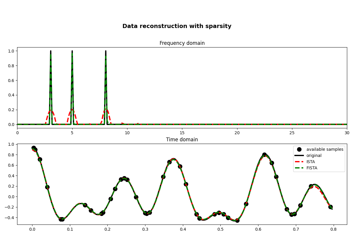
fig, axs = plt.subplots(2, 1, figsize=(12, 8))
fig.suptitle("Data reconstruction with sparsity", fontsize=14, fontweight="bold", y=0.9)
axs[0].plot(f, np.abs(X), "k", lw=3)
axs[0].plot(f, np.abs(pista), "--r", lw=3)
axs[0].plot(f, np.abs(pfista), "--g", lw=3)
axs[0].set_xlim(0, 30)
axs[0].set_title("Frequency domain")
axs[1].plot(t[iava], y, ".k", ms=20, label="available samples")
axs[1].plot(t, x, "k", lw=3, label="original")
axs[1].plot(t, xista, "--r", lw=3, label="ISTA")
axs[1].plot(t, xfista, "--g", lw=3, label="FISTA")
axs[1].set_title("Time domain")
axs[1].axis("tight")
axs[1].legend()
plt.tight_layout()
plt.subplots_adjust(top=0.8)
fig, axs = plt.subplots(2, 1, figsize=(12, 8))
fig.suptitle("Norms history", fontsize=14, fontweight="bold", y=0.9)
axs[0].semilogy(cb.res_perc, "r", lw=3)
axs[0].semilogy(cbf.res_perc, "g", lw=3)
axs[0].set_title("Residual percentage change")
axs[1].semilogy(cb.x_perc, "r", lw=3, label="ISTA")
axs[1].semilogy(cbf.x_perc, "g", lw=3, label="FISTA")
axs[1].set_title("Solution percentage change")
axs[1].legend()
plt.tight_layout()
plt.subplots_adjust(top=0.8)
Total running time of the script: ( 0 minutes 3.739 seconds)