Note
Click here to download the full example code
18. Deblending
The cocktail party problem arises when sounds from different sources mix before reaching our ears (or any recording device), requiring the brain (or any hardware in the recording device) to estimate individual sources from the received mixture. In seismic acquisition, an analog problem is present when multiple sources are fired simultaneously. This family of acquisition methods is usually referred to as simultaneous shooting and the problem of separating the blendend shot gathers into their individual components is called deblending. Whilst various firing strategies can be adopted, in this example we consider the continuos blending problem where a single source is fired sequentially at an interval shorter than the amount of time required for waves to travel into the Earth and come back.
Simply stated the forward problem can be written as:
Here \(\mathbf{d} = [\mathbf{d}_1^T, \mathbf{d}_2^T,\ldots, \mathbf{d}_N^T]^T\) is a stack of \(N\) individual shot gathers, \(\boldsymbol\Phi=[\boldsymbol\Phi_1, \boldsymbol\Phi_2,\ldots, \boldsymbol\Phi_N]\) is the blending operator, \(\mathbf{d}^b\) is the so-called supergather than contains all shots superimposed to each other.
In order to successfully invert this severely underdetermined problem, two key ingredients must be introduced:
the firing time of each source (i.e., shifts of the blending operator) must be chosen to be dithered around a nominal regular, periodic firing interval. In our case, we consider shots of duration \(T=4s\), regular firing time of \(T_s=2s\) and a dithering code as follows \(\Delta t = U(-1,1)\);
prior information about the data to reconstruct, either in the form of regularization or preconditioning must be introduced. In our case we will use a patch-FK transform as preconditioner and solve the problem imposing sparsity in the transformed domain.
In other words, we aim to solve the following problem:
for which we will use the pylops.optimization.sparsity.fista solver.
import matplotlib.pyplot as plt
import numpy as np
from scipy.sparse.linalg import lobpcg as sp_lobpcg

import pylops

np.random.seed(10)
plt.close("all")
Let’s start by defining a blending operator
def Blending(nt, ns, dt, overlap, times, dtype="float64"):
    """Blending operator"""
    pad = int(overlap * nt)
    OpShiftPad = []
    for i in range(ns):
        PadOp = pylops.Pad(nt, (pad * i, pad * (ns - 1 - i)), dtype=dtype)
        ShiftOp = pylops.signalprocessing.Shift(
            pad * (ns - 1) + nt, times[i], axis=0, sampling=dt, real=False, dtype=dtype
        )
        OpShiftPad.append(ShiftOp * PadOp)
    return pylops.HStack(OpShiftPad)
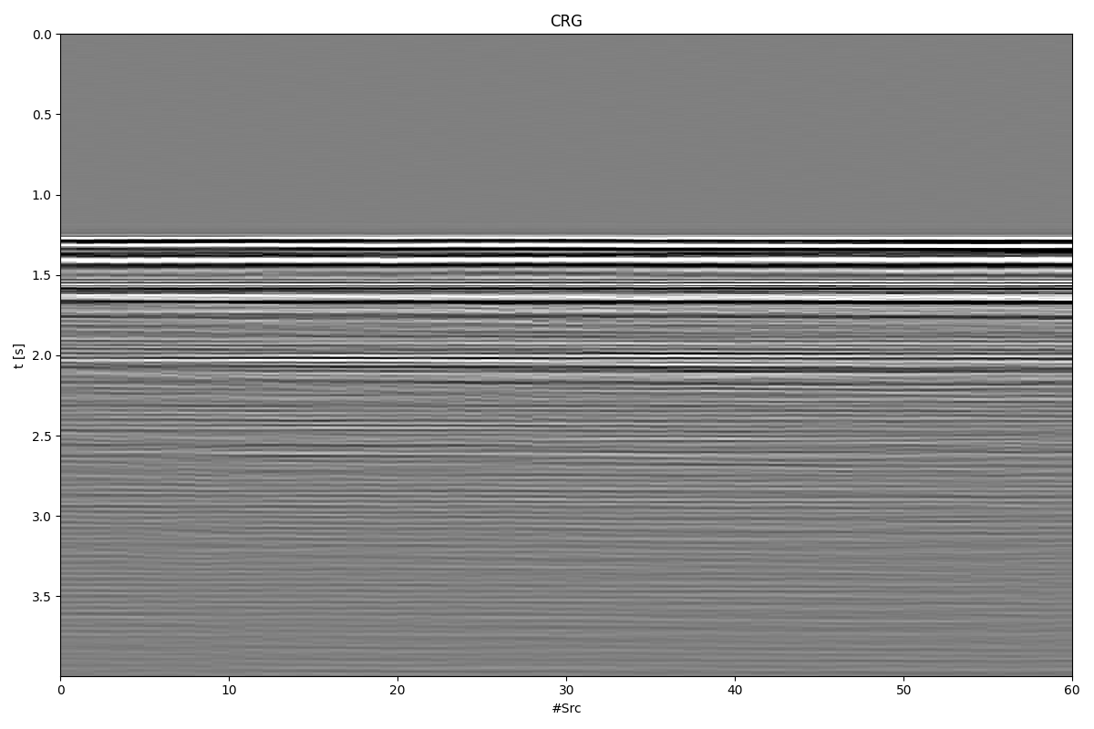
We can now load and display a small portion of the MobilAVO dataset composed of 60 shots and a single receiver. This data is unblended.
data = np.load("../testdata/deblending/mobil.npy")
ns, nt = data.shape

dt = 0.004
t = np.arange(nt) * dt

fig, ax = plt.subplots(1, 1, figsize=(12, 8))
ax.imshow(
    data.T,
    cmap="gray",
    vmin=-50,
    vmax=50,
    extent=(0, ns, t[-1], 0),
    interpolation="none",
)
ax.set_title("CRG")
ax.set_xlabel("#Src")
ax.set_ylabel("t [s]")
ax.axis("tight")
plt.tight_layout()
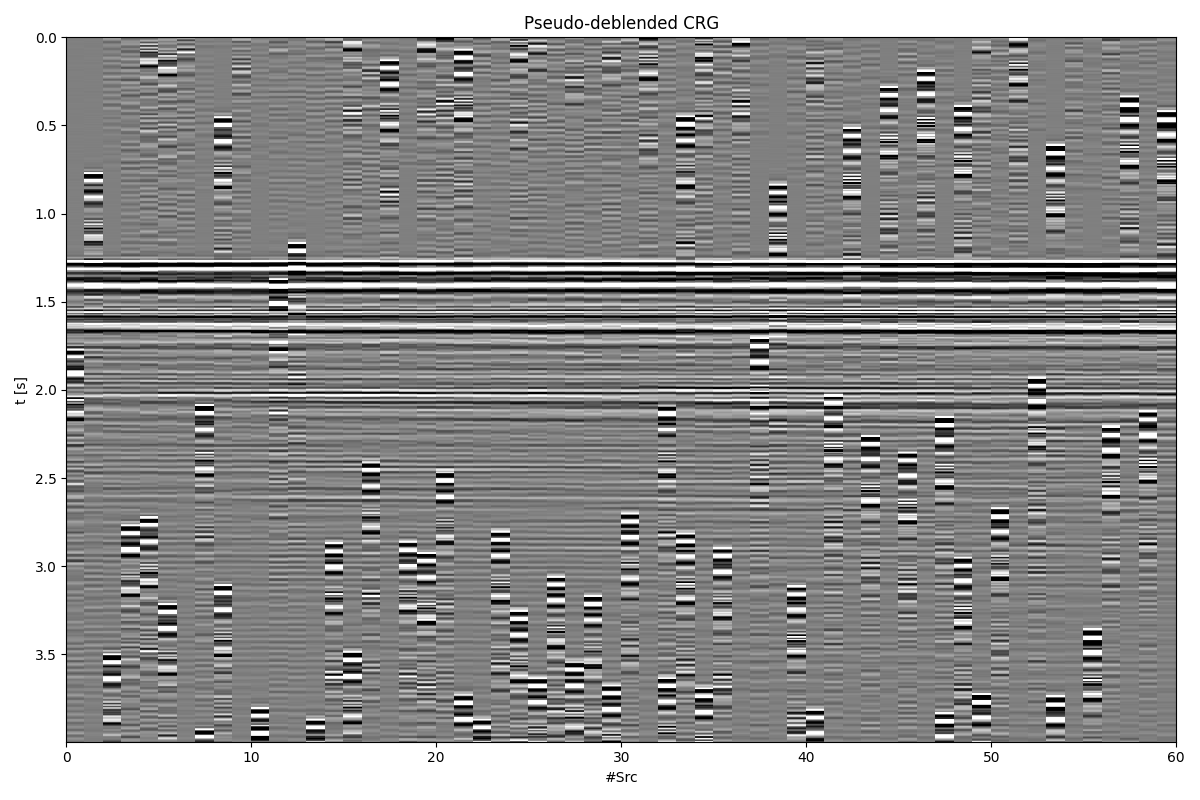
We are now ready to define the blending operator, blend our data, and apply the adjoint of the blending operator to it. This is usually referred as pseudo-deblending: as we will see brings back each source to its own nominal firing time, but since sources partially overlap in time, it will also generate some burst like noise in the data. Deblending can hopefully fix this.
overlap = 0.5
pad = int(overlap * nt)
ignition_times = 2.0 * np.random.rand(ns) - 1.0
Bop = Blending(nt, ns, dt, overlap, ignition_times, dtype="complex128")
data_blended = Bop * data.ravel()
data_pseudo = Bop.H * data_blended.ravel()
data_pseudo = data_pseudo.reshape(ns, nt)

fig, ax = plt.subplots(1, 1, figsize=(12, 8))
ax.imshow(
    data_pseudo.T.real,
    cmap="gray",
    vmin=-50,
    vmax=50,
    extent=(0, ns, t[-1], 0),
    interpolation="none",
)
ax.set_title("Pseudo-deblended CRG")
ax.set_xlabel("#Src")
ax.set_ylabel("t [s]")
ax.axis("tight")
plt.tight_layout()
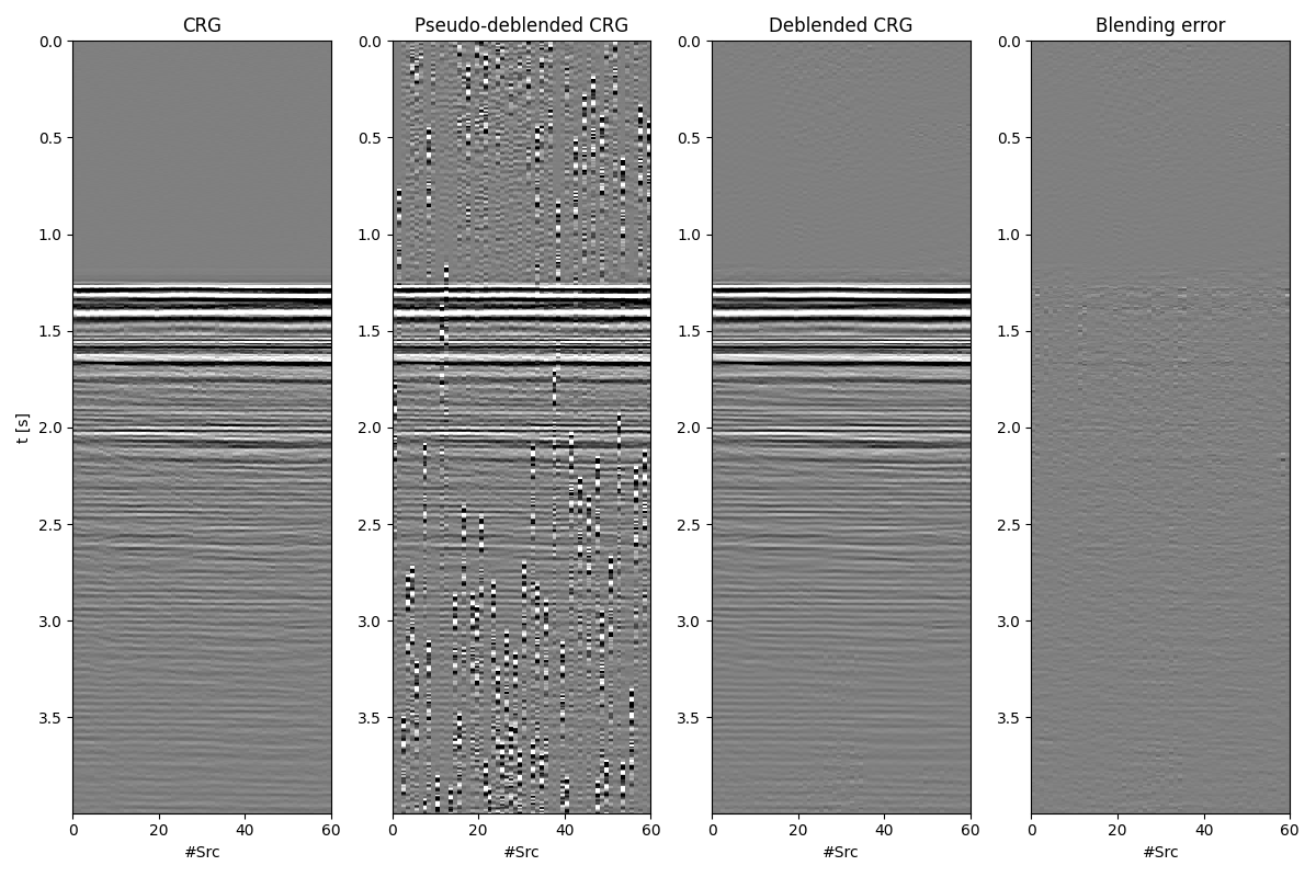
We are finally ready to solve our deblending inverse problem
# Patched FK
dimsd = data.shape
nwin = (20, 80)
nover = (10, 40)
nop = (128, 128)
nop1 = (128, 65)
nwins = (5, 24)
dims = (nwins[0] * nop1[0], nwins[1] * nop1[1])

Fop = pylops.signalprocessing.FFT2D(nwin, nffts=nop, real=True)
Sop = pylops.signalprocessing.Patch2D(
    Fop.H, dims, dimsd, nwin, nover, nop1, tapertype="hanning"
)
# Overall operator
Op = Bop * Sop

# Compute max eigenvalue (we do this explicitly to be able to run this fast)
Op1 = pylops.LinearOperator(Op.H * Op, explicit=False)
X = np.random.rand(Op1.shape[0], 1).astype(Op1.dtype)
maxeig = sp_lobpcg(Op1, X=X, maxiter=5, tol=1e-10)[0][0]
alpha = 1.0 / maxeig

# Deblend
niter = 60
decay = (np.exp(-0.05 * np.arange(niter)) + 0.2) / 1.2

with pylops.disabled_ndarray_multiplication():
    p_inv = pylops.optimization.sparsity.fista(
        Op,
        data_blended.ravel(),
        niter=niter,
        eps=5e0,
        alpha=alpha,
        decay=decay,
        show=True,
    )[0]
data_inv = Sop * p_inv
data_inv = data_inv.reshape(ns, nt)

fig, axs = plt.subplots(1, 4, sharey=False, figsize=(12, 8))
axs[0].imshow(
    data.T.real,
    cmap="gray",
    extent=(0, ns, t[-1], 0),
    vmin=-50,
    vmax=50,
    interpolation="none",
)
axs[0].set_title("CRG")
axs[0].set_xlabel("#Src")
axs[0].set_ylabel("t [s]")
axs[0].axis("tight")
axs[1].imshow(
    data_pseudo.T.real,
    cmap="gray",
    extent=(0, ns, t[-1], 0),
    vmin=-50,
    vmax=50,
    interpolation="none",
)
axs[1].set_title("Pseudo-deblended CRG")
axs[1].set_xlabel("#Src")
axs[1].axis("tight")
axs[2].imshow(
    data_inv.T.real,
    cmap="gray",
    extent=(0, ns, t[-1], 0),
    vmin=-50,
    vmax=50,
    interpolation="none",
)
axs[2].set_xlabel("#Src")
axs[2].set_title("Deblended CRG")
axs[2].axis("tight")
axs[3].imshow(
    data.T.real - data_inv.T.real,
    cmap="gray",
    extent=(0, ns, t[-1], 0),
    vmin=-50,
    vmax=50,
    interpolation="none",
)
axs[3].set_xlabel("#Src")
axs[3].set_title("Blending error")
axs[3].axis("tight")
plt.tight_layout()
FISTA (soft thresholding)
--------------------------------------------------------------------------------
The Operator Op has 30500 rows and 998400 cols
eps = 5.000000e+00      tol = 1.000000e-10      niter = 60
alpha = 3.261681e-01    thresh = 8.154204e-01
--------------------------------------------------------------------------------
   Itn          x[0]              r2norm     r12norm     xupdate
     1   0.00e+00+0.00e+00j    3.463e+06   5.081e+06   1.251e+03
     2   0.00e+00+0.00e+00j    1.955e+06   4.282e+06   6.844e+02
     3   0.00e+00+0.00e+00j    1.134e+06   3.898e+06   5.635e+02
     4   0.00e+00+0.00e+00j    7.080e+05   3.681e+06   4.576e+02
     5   0.00e+00+0.00e+00j    4.873e+05   3.510e+06   3.831e+02
     6   0.00e+00+0.00e+00j    3.688e+05   3.348e+06   3.357e+02
     7   0.00e+00+0.00e+00j    3.014e+05   3.192e+06   3.048e+02
     8   0.00e+00+0.00e+00j    2.600e+05   3.048e+06   2.826e+02
     9   0.00e+00+0.00e+00j    2.316e+05   2.923e+06   2.642e+02
    10   0.00e+00+0.00e+00j    2.105e+05   2.816e+06   2.479e+02
    11   0.00e+00+0.00e+00j    1.934e+05   2.727e+06   2.327e+02
    21   0.00e+00+0.00e+00j    1.028e+05   2.435e+06   1.202e+02
    31   -0.00e+00+0.00e+00j    6.359e+04   2.450e+06   8.024e+01
    41   -0.00e+00+0.00e+00j    4.281e+04   2.490e+06   6.262e+01
    51   -0.00e+00+0.00e+00j    3.179e+04   2.520e+06   5.211e+01
    52   -0.00e+00+0.00e+00j    3.101e+04   2.523e+06   5.126e+01
    53   -0.00e+00+0.00e+00j    3.027e+04   2.525e+06   5.040e+01
    54   -0.00e+00+0.00e+00j    2.957e+04   2.527e+06   4.960e+01
    55   -0.00e+00+0.00e+00j    2.890e+04   2.529e+06   4.879e+01
    56   -0.00e+00+0.00e+00j    2.827e+04   2.531e+06   4.804e+01
    57   -0.00e+00+0.00e+00j    2.768e+04   2.533e+06   4.733e+01
    58   -0.00e+00+0.00e+00j    2.712e+04   2.535e+06   4.663e+01
    59   -0.00e+00+0.00e+00j    2.660e+04   2.536e+06   4.598e+01
    60   -0.00e+00+0.00e+00j    2.610e+04   2.538e+06   4.531e+01

Iterations = 60        Total time (s) = 44.24
--------------------------------------------------------------------------------
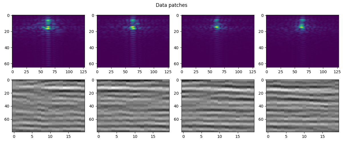
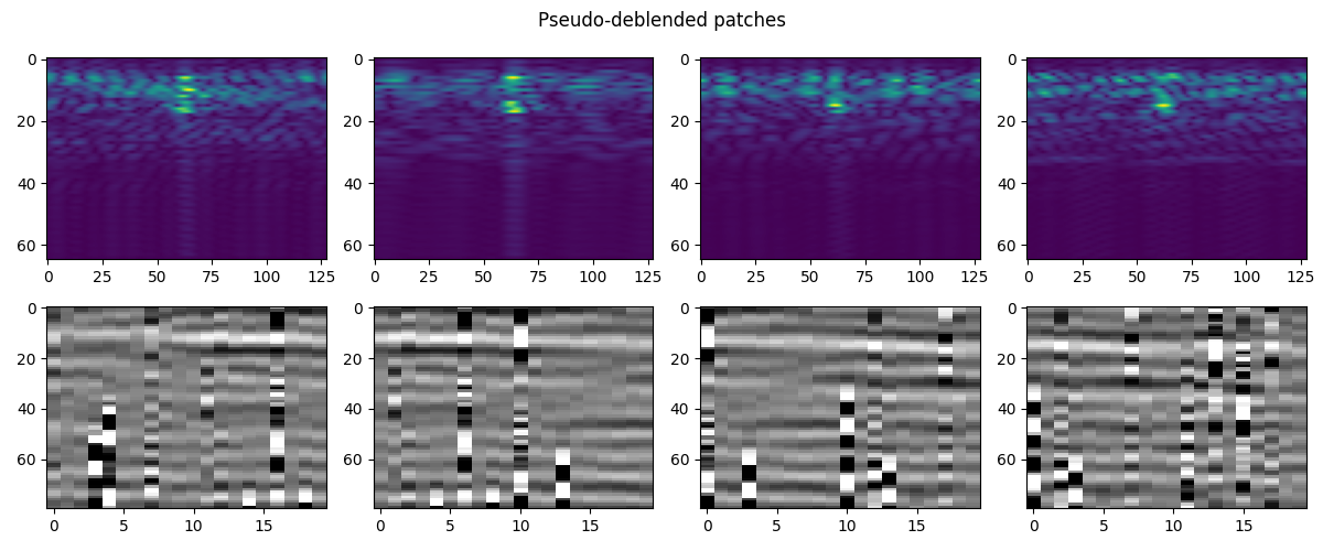
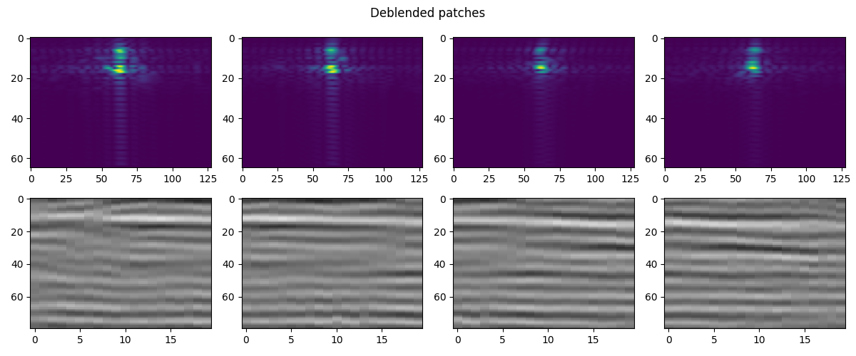
Finally, let’s look a bit more at what really happened under the hood. We display a number of patches and their associated FK spectrum
Sop1 = pylops.signalprocessing.Patch2D(
    Fop.H, dims, dimsd, nwin, nover, nop1, tapertype=None
)

# Original
p = Sop1.H * data.ravel()
preshape = p.reshape(nwins[0], nwins[1], nop1[0], nop1[1])

ix = 16
fig, axs = plt.subplots(2, 4, figsize=(12, 5))
fig.suptitle("Data patches")
for i in range(4):
    axs[0][i].imshow(np.fft.fftshift(np.abs(preshape[i, ix]).T, axes=1))
    axs[0][i].axis("tight")
    axs[1][i].imshow(
        np.real((Fop.H * preshape[i, ix].ravel()).reshape(nwin)).T,
        cmap="gray",
        vmin=-30,
        vmax=30,
        interpolation="none",
    )
    axs[1][i].axis("tight")
plt.tight_layout()

# Pseudo-deblended
p_pseudo = Sop1.H * data_pseudo.ravel()
p_pseudoreshape = p_pseudo.reshape(nwins[0], nwins[1], nop1[0], nop1[1])

ix = 16
fig, axs = plt.subplots(2, 4, figsize=(12, 5))
fig.suptitle("Pseudo-deblended patches")
for i in range(4):
    axs[0][i].imshow(np.fft.fftshift(np.abs(p_pseudoreshape[i, ix]).T, axes=1))
    axs[0][i].axis("tight")
    axs[1][i].imshow(
        np.real((Fop.H * p_pseudoreshape[i, ix].ravel()).reshape(nwin)).T,
        cmap="gray",
        vmin=-30,
        vmax=30,
        interpolation="none",
    )
    axs[1][i].axis("tight")
plt.tight_layout()

# Deblended
p_inv = Sop1.H * data_inv.ravel()
p_invreshape = p_inv.reshape(nwins[0], nwins[1], nop1[0], nop1[1])

ix = 16
fig, axs = plt.subplots(2, 4, figsize=(12, 5))
fig.suptitle("Deblended patches")
for i in range(4):
    axs[0][i].imshow(np.fft.fftshift(np.abs(p_invreshape[i, ix]).T, axes=1))
    axs[0][i].axis("tight")
    axs[1][i].imshow(
        np.real((Fop.H * p_invreshape[i, ix].ravel()).reshape(nwin)).T,
        cmap="gray",
        vmin=-30,
        vmax=30,
        interpolation="none",
    )
    axs[1][i].axis("tight")
plt.tight_layout()
Total running time of the script: ( 0 minutes 51.398 seconds)