Note
Click here to download the full example code
01. The LinearOpeator
This first tutorial is aimed at easing the use of the PyLops library for both new users and developers.
Since PyLops heavily relies on the use of the
scipy.sparse.linalg.LinearOperator class of SciPy, we will start
by looking at how to initialize a linear operator as well as
different ways to apply the forward and adjoint operations. Finally we will
investigate various special methods, also called magic methods
(i.e., methods with the double underscores at the beginning and the end) that
have been implemented for such a class and will allow summing, subtractring,
chaining, etc. multiple operators in very easy and expressive way.
Let’s start by defining a simple operator that applies element-wise
multiplication of the model with a vector d in forward mode and
element-wise multiplication of the data with the same vector d in
adjoint mode. This operator is present in PyLops under the
name of pylops.Diagonal and
its implementation is discussed in more details in the Implementing new operators
page.
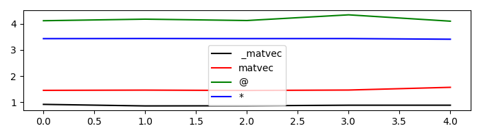
First of all we apply the operator in the forward mode. This can be done in four different ways:
_matvec: directly applies the method implemented for forward modematvec: performs some checks before and after applying_matvec*: operator used to map the special method__matmul__which checks whether the inputxis a vector or matrix and applies_matvecor_matmulaccordingly.@: operator used to map the special method__mul__which performs like the*opetator
We will time these 4 different executions and see how using _matvec
(or matvec) will result in the faster computation. It is thus advised to
use * (or @) in examples when expressivity has priority but prefer
_matvec (or matvec) for efficient implementations.
# setup command
cmd_setup = """\
import numpy as np
import pylops
n = 10
d = np.arange(n) + 1.
x = np.ones(n)
Dop = pylops.Diagonal(d)
DopH = Dop.H
"""

# _matvec
cmd1 = "Dop._matvec(x)"

# matvec
cmd2 = "Dop.matvec(x)"

# @
cmd3 = "Dop@x"

# *
cmd4 = "Dop*x"

# timing
t1 = 1.0e3 * np.array(timeit.repeat(cmd1, setup=cmd_setup, number=500, repeat=5))
t2 = 1.0e3 * np.array(timeit.repeat(cmd2, setup=cmd_setup, number=500, repeat=5))
t3 = 1.0e3 * np.array(timeit.repeat(cmd3, setup=cmd_setup, number=500, repeat=5))
t4 = 1.0e3 * np.array(timeit.repeat(cmd4, setup=cmd_setup, number=500, repeat=5))

plt.figure(figsize=(7, 2))
plt.plot(t1, "k", label=" _matvec")
plt.plot(t2, "r", label="matvec")
plt.plot(t3, "g", label="@")
plt.plot(t4, "b", label="*")
plt.axis("tight")
plt.legend()
plt.tight_layout()
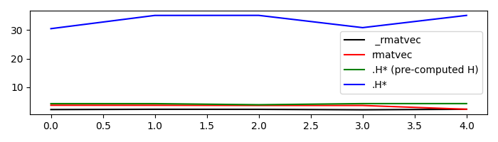
Similarly we now consider the adjoint mode. This can be done in three different ways:
_rmatvec: directly applies the method implemented for adjoint modermatvec: performs some checks before and after applying_rmatvec.H*: first applies the adjoint.Hwhich creates a new scipy.sparse.linalg._CustomLinearOperator` where_matvecand_rmatvecare swapped and then applies the new_matvec.
Once again, after timing these 3 different executions we can see
see how using _rmatvec (or rmatvec) will result in the faster
computation while .H* is very unefficient and slow. Note that if the
adjoint has to be applied multiple times it is at least advised to create
the adjoint operator by applying .H only once upfront.
Not surprisingly, the linear solvers in scipy as well as in PyLops
actually use matvec and rmatvec when dealing with linear operators.
# _rmatvec
cmd1 = "Dop._rmatvec(x)"

# rmatvec
cmd2 = "Dop.rmatvec(x)"

# .H* (pre-computed H)
cmd3 = "DopH*x"

# .H*
cmd4 = "Dop.H*x"

# timing
t1 = 1.0e3 * np.array(timeit.repeat(cmd1, setup=cmd_setup, number=500, repeat=5))
t2 = 1.0e3 * np.array(timeit.repeat(cmd2, setup=cmd_setup, number=500, repeat=5))
t3 = 1.0e3 * np.array(timeit.repeat(cmd3, setup=cmd_setup, number=500, repeat=5))
t4 = 1.0e3 * np.array(timeit.repeat(cmd4, setup=cmd_setup, number=500, repeat=5))

plt.figure(figsize=(7, 2))
plt.plot(t1, "k", label=" _rmatvec")
plt.plot(t2, "r", label="rmatvec")
plt.plot(t3, "g", label=".H* (pre-computed H)")
plt.plot(t4, "b", label=".H*")
plt.axis("tight")
plt.legend()
plt.tight_layout()
Just to reiterate once again, it is advised to call matvec
and rmatvec unless PyLops linear operators are used for
teaching purposes.
We now go through some other methods and special methods that
are implemented in scipy.sparse.linalg.LinearOperator (and
pylops.LinearOperator):
Op1+Op2: maps the special method__add__and performs summation between two operators and returns apylops.LinearOperator-Op: maps the special method__neg__and performs negation of an operators and returns apylops.LinearOperatorOp1-Op2: maps the special method__sub__and performs summation between two operators and returns apylops.LinearOperatorOp1**N: maps the special method__pow__and performs exponentiation of an operator and returns apylops.LinearOperatorOp/y(andOp.div(y)): maps the special method__truediv__and performs inversion of an operatorOp.eigs(): estimates the eigenvalues of the operatorOp.cond(): estimates the condition number of the operatorOp.conj(): create complex conjugate operator
<10x10 LinearOperator with dtype=float64>
<10x10 LinearOperator with dtype=float64>
<10x10 LinearOperator with dtype=float64>
<10x10 LinearOperator with dtype=float64>
[1. 1. 1. 1. 1. 1. 1. 1. 1. 1.]
[10.+0.j  9.+0.j  8.+0.j]
(10.00000000000003+0j)
<10x10 _ConjLinearOperator with dtype=float64>
To understand the effect of conj we need to look into a problem with an
operator in the complex domain. Let’s create again our
pylops.Diagonal operator but this time we populate it with
complex numbers. We will see that the action of the operator and its complex
conjugate is different even if the model is real.
y = Dx = [0.+1.j 0.+2.j 0.+3.j 0.+4.j 0.+5.j]
y = conj(D)x = [0.-1.j 0.-2.j 0.-3.j 0.-4.j 0.-5.j]
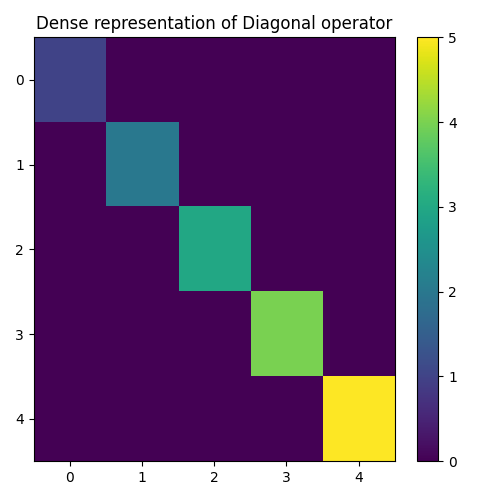
At this point, the concept of linear operator may sound abstract.
The convinience method pylops.LinearOperator.todense can be used to
create the equivalent dense matrix of any operator. In this case for example
we expect to see a diagonal matrix with d values along the main diagonal
D = Dop.todense()

plt.figure(figsize=(5, 5))
plt.imshow(np.abs(D))
plt.title("Dense representation of Diagonal operator")
plt.axis("tight")
plt.colorbar()
plt.tight_layout()
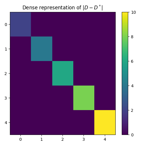
At this point it is worth reiterating that if two linear operators are
combined by means of the algebraical operations shown above, the resulting
operator is still a pylops.LinearOperator operator. This means
that we can still apply any of the methods implemented in the original
scipy class definition like *, as well as those in our class
definition like /
Dop1 = Dop - Dop.conj()

y = Dop1 * x
print(f"x = (Dop - conj(Dop))/y = {Dop1 / y}")

D1 = Dop1.todense()

plt.figure(figsize=(5, 5))
plt.imshow(np.abs(D1))
plt.title(r"Dense representation of $|D - D^*|$")
plt.axis("tight")
plt.colorbar()
plt.tight_layout()
x = (Dop - conj(Dop))/y = [1.+0.j 1.+0.j 1.+0.j 1.+0.j 1.+0.j]
Finally, another important feature of PyLops linear operators is that we can always keep track of how many times the forward and adjoint passes have been applied (and reset when needed). This is particularly useful when running a third party solver to see how many evaluations of our operator are performed inside the solver.
Dop = pylops.Diagonal(d)

y = Dop.matvec(x)
y = Dop.matvec(x)
y = Dop.rmatvec(y)

print(f"Forward evaluations: {Dop.matvec_count}")
print(f"Adjoint evaluations: {Dop.rmatvec_count}")

# Reset
Dop.reset_count()
print(f"Forward evaluations: {Dop.matvec_count}")
print(f"Adjoint evaluations: {Dop.rmatvec_count}")
Forward evaluations: 2
Adjoint evaluations: 1
Forward evaluations: 0
Adjoint evaluations: 0
This first tutorial is completed. You have seen the basic operations that
can be performed using scipy.sparse.linalg.LinearOperator and
our overload of such a class pylops.LinearOperator and you
should be able to get started combining various PyLops operators and
solving your own inverse problems.
Total running time of the script: ( 0 minutes 1.049 seconds)