pylops.utils.signalprocessing.slope_estimate

pylops.utils.signalprocessing.slope_estimate(d, dz=1.0, dx=1.0, smooth=5.0, eps=0.0, dips=False)

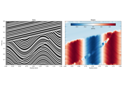
Local slope estimation

Local slopes are estimated using the Structure Tensor algorithm [1]. Slopes are returned as \(\tan\theta\), defined in a RHS coordinate system with \(z\)-axis pointing upward.

Note

For stability purposes, it is important to ensure that the orders of magnitude of the samplings are similar.

Parameters:

dnumpy.ndarray

Input dataset of size \(n_z \times n_x\)

dzfloat, optional

Sampling in \(z\)-axis, \(\Delta z\)

Warning

Since version 1.17.0, defaults to 1.0.

dxfloat, optional

Sampling in \(x\)-axis, \(\Delta x\)

Warning

Since version 1.17.0, defaults to 1.0.

smoothfloat or numpy.ndarray, optional

Standard deviation for Gaussian kernel. The standard deviations of the Gaussian filter are given for each axis as a sequence, or as a single number, in which case it is equal for all axes.

Warning

Default changed in version 1.17.0 to 5 from previous value of 20.

epsfloat, optional

Added in version 1.17.0.

Regularization term. All slopes where \(|g_{zx}| < \epsilon \max_{(x, z)} \{|g_{zx}|, |g_{zz}|, |g_{xx}|\}\) are set to zero. All anisotropies where \(\lambda_\text{max} < \epsilon\) are also set to zero. See Notes. When using with small values of smooth, start from a very small number (e.g. 1e-10) and start increasing by a power of 10 until results are satisfactory.

dipsbool, optional

Added in version 2.0.0.

Return dips (True) instead of slopes (False).

Returns:

slopesnumpy.ndarray

Estimated local slopes. The unit is that of \(\Delta z/\Delta x\).

Warning

Prior to version 1.17.0, always returned dips.

anisotropiesnumpy.ndarray

Estimated local anisotropies: \(1-\lambda_\text{min}/\lambda_\text{max}\)

Note

Since 1.17.0, changed name from linearity to anisotropies. Definition remains the same.

Notes

For each pixel of the input dataset \(\mathbf{d}\) the local gradients \(g_z = \frac{\partial \mathbf{d}}{\partial z}\) and \(g_x = \frac{\partial \mathbf{d}}{\partial x}\) are computed and used to define the following three quantities:

\[\begin{split}\begin{align} g_{zz} &= \left(\frac{\partial \mathbf{d}}{\partial z}\right)^2\\ g_{xx} &= \left(\frac{\partial \mathbf{d}}{\partial x}\right)^2\\ g_{zx} &= \frac{\partial \mathbf{d}}{\partial z}\cdot\frac{\partial \mathbf{d}}{\partial x} \end{align}\end{split}\]

They are then spatially smoothed and at each pixel their smoothed versions are arranged in a \(2 \times 2\) matrix called the smoothed gradient-square tensor:

\[\begin{split}\mathbf{G} = \begin{bmatrix} g_{zz} & g_{zx} \\ g_{zx} & g_{xx} \end{bmatrix}\end{split}\]

Local slopes can be expressed as \(p = \frac{\lambda_\text{max} - g_{zz}}{g_{zx}}\), where \(\lambda_\text{max}\) is the largest eigenvalue of \(\mathbf{G}\).

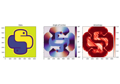
Similarly, local dips can be expressed as \(\tan(2\theta) = 2g_{zx} / (g_{zz} - g_{xx})\).

Moreover, we can obtain a measure of local anisotropy, defined as

\[a = 1-\lambda_\text{min}/\lambda_\text{max}\]

where \(\lambda_\text{min}\) is the smallest eigenvalue of \(\mathbf{G}\). A value of \(a = 0\) indicates perfect isotropy whereas \(a = 1\) indicates perfect anisotropy.

[1]

Van Vliet, L. J., Verbeek, P. W., “Estimators for orientation and anisotropy in digitized images”, Journal ASCI Imaging Workshop. 1995.

Examples using pylops.utils.signalprocessing.slope_estimate

PWD-based slope estimation and structural smoothing

PWD-based slope estimation and structural smoothing

Seislet transform

Seislet transform

Slope estimation via Structure Tensor algorithm

Slope estimation via Structure Tensor algorithm