Slope estimation via Structure Tensor algorithm¶

This example shows how to estimate local slopes or local dips of two- or three-dimensional arrays using pylops.utils.signalprocessing.slope_estimate and pylops.utils.signalprocessing.dip_estimate.

Knowing the local slopes of an image (or a seismic data) can be useful for a variety of tasks in image (or geophysical) processing such as denoising, smoothing, or interpolation. When slopes are used with the pylops.signalprocessing.Seislet operator, the input dataset can be compressed and the sparse nature of the Seislet transform can also be used to precondition sparsity-promoting inverse problems.

We will show examples of a variety of different settings, including a comparison with the original implementation in [1].

import matplotlib.pyplot as plt
import numpy as np
from matplotlib.image import imread
from matplotlib.ticker import FuncFormatter, MultipleLocator
from mpl_toolkits.axes_grid1 import make_axes_locatable

import pylops
from pylops.signalprocessing.seislet import _predict_trace
from pylops.utils.signalprocessing import dip_estimate, slope_estimate

plt.close("all")
np.random.seed(10)


def create_colorbar(fig, ax, im):
    divider = make_axes_locatable(ax)
    cax = divider.append_axes("right", size="5%", pad=0.1)
    cb = fig.colorbar(im, cax=cax, orientation="vertical")
    return cax, cb

Python logo¶

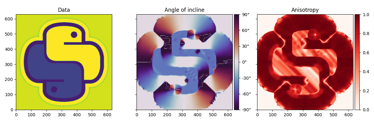
To start we import a 2d image and estimate the local dips of the image.

im = np.load("../testdata/python.npy")[..., 0]
im = im / 255.0 - 0.5

angles, anisotropy = dip_estimate(im, smooth=7)
angles = -np.rad2deg(angles)

fig, axs = plt.subplots(1, 3, figsize=(12, 4), sharex=True, sharey=True)
iax = axs[0].imshow(im, cmap="viridis", origin="lower")
axs[0].set_title("Data")
cax = make_axes_locatable(axs[0]).append_axes("right", size="5%", pad=0.05)
cax.axis("off")

iax = axs[1].imshow(angles, cmap="twilight_shifted", origin="lower", vmin=-90, vmax=90)
axs[1].set_title("Angle of incline")
cax = make_axes_locatable(axs[1]).append_axes("right", size="5%", pad=0.05)
cb = fig.colorbar(
    iax,
    ticks=MultipleLocator(30),
    format=FuncFormatter(lambda x, pos: f"{x:.0f}°"),
    cax=cax,
    orientation="vertical",
)

iax = axs[2].imshow(anisotropy, cmap="Reds", origin="lower", vmin=0, vmax=1)
axs[2].set_title("Anisotropy")
cax = make_axes_locatable(axs[2]).append_axes("right", size="5%", pad=0.05)
cb = fig.colorbar(iax, cax=cax, orientation="vertical")
fig.tight_layout()

Seismic data¶

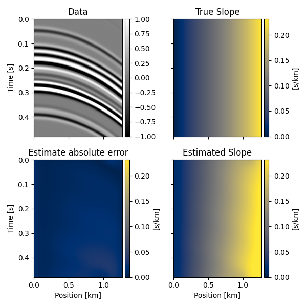
We can now repeat the same using some seismic data. We will first define a single trace and a slope field, apply such slope field to the trace recursively to create the other traces of the data and finally try to recover the underlying slope field from the data alone.

# Reflectivity model
nx, nt = 2**7, 121
dx, dt = 0.01, 0.004
x, t = np.arange(nx) * dx, np.arange(nt) * dt

nspike = nt // 8
refl = np.zeros(nt)
it = np.sort(np.random.permutation(range(10, nt - 20))[:nspike])
refl[it] = np.random.normal(0.0, 1.0, nspike)

# Wavelet
ntwav = 41
f0 = 30
twav = np.arange(ntwav) * dt
wav, *_ = pylops.utils.wavelets.ricker(twav, f0)

# Input trace
trace = np.convolve(refl, wav, mode="same")

# Slopes
theta = np.deg2rad(np.linspace(0, 30, nx))
slope = np.outer(np.ones(nt), np.tan(theta) * dt / dx)

# Model data
d = np.zeros((nt, nx))
tr = trace.copy()
for ix in range(nx):
    tr = _predict_trace(tr, t, dt, dx, slope[:, ix])
    d[:, ix] = tr

# Estimate slopes
slope_est, _ = slope_estimate(d, dt, dx, smooth=10)
slope_est *= -1

fig, axs = plt.subplots(2, 2, figsize=(6, 6), sharex=True, sharey=True)

opts = dict(aspect="auto", extent=(x[0], x[-1], t[-1], t[0]))
iax = axs[0, 0].imshow(d, cmap="gray", vmin=-1, vmax=1, **opts)
axs[0, 0].set(title="Data", ylabel="Time [s]")
cax = make_axes_locatable(axs[0, 0]).append_axes("right", size="5%", pad=0.05)
fig.colorbar(iax, cax=cax, orientation="vertical")

opts.update(dict(cmap="cividis", vmin=np.min(slope), vmax=np.max(slope)))
iax = axs[0, 1].imshow(slope, **opts)
axs[0, 1].set(title="True Slope")
cax = make_axes_locatable(axs[0, 1]).append_axes("right", size="5%", pad=0.05)
fig.colorbar(iax, cax=cax, orientation="vertical")
cax.set_ylabel("[s/km]")

iax = axs[1, 0].imshow(np.abs(slope - slope_est), **opts)
axs[1, 0].set(
    title="Estimate absolute error", ylabel="Time [s]", xlabel="Position [km]"
)
cax = make_axes_locatable(axs[1, 0]).append_axes("right", size="5%", pad=0.05)
fig.colorbar(iax, cax=cax, orientation="vertical")
cax.set_ylabel("[s/km]")

iax = axs[1, 1].imshow(slope_est, **opts)
axs[1, 1].set(title="Estimated Slope", xlabel="Position [km]")
cax = make_axes_locatable(axs[1, 1]).append_axes("right", size="5%", pad=0.05)
fig.colorbar(iax, cax=cax, orientation="vertical")
cax.set_ylabel("[s/km]")

fig.tight_layout()

Data, True Slope, Estimate absolute error, Estimated Slope

Concentric circles¶

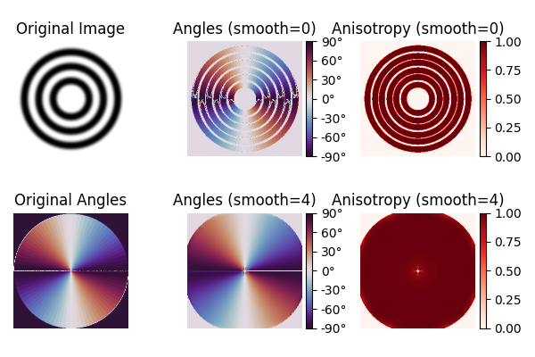
The original paper by van Vliet and Verbeek [1] has an example with concentric circles. We recover their original images and compare our implementation with theirs.

def rgb2gray(rgb):
    return np.dot(rgb[..., :3], [0.2989, 0.5870, 0.1140])


circles_input = rgb2gray(imread("../testdata/slope_estimate/concentric.png"))
circles_angles = rgb2gray(imread("../testdata/slope_estimate/concentric_angles.png"))

angles, anisos_sm0 = dip_estimate(circles_input, smooth=0)
angles_sm0 = np.rad2deg(angles)

angles, anisos_sm4 = dip_estimate(circles_input, smooth=4)
angles_sm4 = np.rad2deg(angles)

fig, axs = plt.subplots(2, 3, figsize=(6, 4), sharex=True, sharey=True)
axs[0, 0].imshow(circles_input, cmap="gray", aspect="equal")
axs[0, 0].set(title="Original Image")
cax = make_axes_locatable(axs[0, 0]).append_axes("right", size="5%", pad=0.05)
cax.axis("off")

axs[1, 0].imshow(-circles_angles, cmap="twilight_shifted")
axs[1, 0].set(title="Original Angles")
cax = make_axes_locatable(axs[1, 0]).append_axes("right", size="5%", pad=0.05)
cax.axis("off")

im = axs[0, 1].imshow(angles_sm0, cmap="twilight_shifted", vmin=-90, vmax=90)
cax = make_axes_locatable(axs[0, 1]).append_axes("right", size="5%", pad=0.05)
cb = fig.colorbar(
    im,
    ticks=MultipleLocator(30),
    format=FuncFormatter(lambda x, pos: f"{x:.0f}°"),
    cax=cax,
    orientation="vertical",
)
axs[0, 1].set(title="Angles (smooth=0)")

im = axs[1, 1].imshow(angles_sm4, cmap="twilight_shifted", vmin=-90, vmax=90)
cax = make_axes_locatable(axs[1, 1]).append_axes("right", size="5%", pad=0.05)
cb = fig.colorbar(
    im,
    ticks=MultipleLocator(30),
    format=FuncFormatter(lambda x, pos: f"{x:.0f}°"),
    cax=cax,
    orientation="vertical",
)
axs[1, 1].set(title="Angles (smooth=4)")

im = axs[0, 2].imshow(anisos_sm0, cmap="Reds", vmin=0, vmax=1)
cax = make_axes_locatable(axs[0, 2]).append_axes("right", size="5%", pad=0.05)
cb = fig.colorbar(im, cax=cax, orientation="vertical")
axs[0, 2].set(title="Anisotropy (smooth=0)")

im = axs[1, 2].imshow(anisos_sm4, cmap="Reds", vmin=0, vmax=1)
cax = make_axes_locatable(axs[1, 2]).append_axes("right", size="5%", pad=0.05)
cb = fig.colorbar(im, cax=cax, orientation="vertical")
axs[1, 2].set(title="Anisotropy (smooth=4)")

for ax in axs.ravel():
    ax.axis("off")
fig.tight_layout()

Original Image, Angles (smooth=0), Anisotropy (smooth=0), Original Angles, Angles (smooth=4), Anisotropy (smooth=4)

Core samples¶

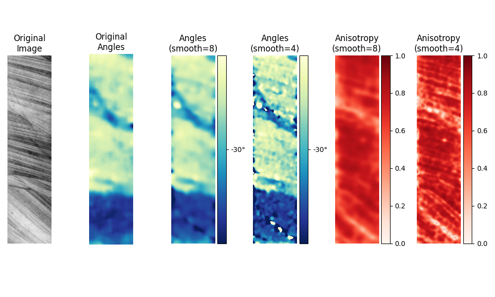
The original paper by van Vliet and Verbeek [1] also has an example with images of core samples. Since the original paper does not have a scale with which to plot the angles, we have chosen ours it to match their image as closely as possible.

core_input = rgb2gray(imread("../testdata/slope_estimate/core_sample.png"))
core_angles = rgb2gray(imread("../testdata/slope_estimate/core_sample_orientation.png"))
core_aniso = rgb2gray(imread("../testdata/slope_estimate/core_sample_anisotropy.png"))


angles, anisos_sm4 = dip_estimate(core_input, smooth=4)
angles_sm4 = np.rad2deg(angles)

angles, anisos_sm8 = dip_estimate(core_input, smooth=8)
angles_sm8 = np.rad2deg(angles)

fig, axs = plt.subplots(1, 6, figsize=(10, 6))

axs[0].imshow(core_input, cmap="gray_r", aspect="equal")
axs[0].set(title="Original\nImage")
cax = make_axes_locatable(axs[0]).append_axes("right", size="20%", pad=0.05)
cax.axis("off")

axs[1].imshow(-core_angles, cmap="YlGnBu_r")
axs[1].set(title="Original\nAngles")
cax = make_axes_locatable(axs[1]).append_axes("right", size="20%", pad=0.05)
cax.axis("off")

im = axs[2].imshow(angles_sm8, cmap="YlGnBu_r", vmin=-49, vmax=-11)
cax = make_axes_locatable(axs[2]).append_axes("right", size="20%", pad=0.05)
cb = fig.colorbar(
    im,
    ticks=MultipleLocator(30),
    format=FuncFormatter(lambda x, pos: f"{x:.0f}°"),
    cax=cax,
    orientation="vertical",
)
axs[2].set(title="Angles\n(smooth=8)")

im = axs[3].imshow(angles_sm4, cmap="YlGnBu_r", vmin=-49, vmax=-11)
cax = make_axes_locatable(axs[3]).append_axes("right", size="20%", pad=0.05)
cb = fig.colorbar(
    im,
    ticks=MultipleLocator(30),
    format=FuncFormatter(lambda x, pos: f"{x:.0f}°"),
    cax=cax,
    orientation="vertical",
)
axs[3].set(title="Angles\n(smooth=4)")

im = axs[4].imshow(anisos_sm8, cmap="Reds", vmin=0, vmax=1)
cax = make_axes_locatable(axs[4]).append_axes("right", size="20%", pad=0.05)
cb = fig.colorbar(im, cax=cax, orientation="vertical")
axs[4].set(title="Anisotropy\n(smooth=8)")

im = axs[5].imshow(anisos_sm4, cmap="Reds", vmin=0, vmax=1)
cax = make_axes_locatable(axs[5]).append_axes("right", size="20%", pad=0.05)
cb = fig.colorbar(im, cax=cax, orientation="vertical")
axs[5].set(title="Anisotropy\n(smooth=4)")

for ax in axs.ravel():
    ax.axis("off")
fig.tight_layout()

Original Image, Original Angles, Angles (smooth=8), Angles (smooth=4), Anisotropy (smooth=8), Anisotropy (smooth=4)

3D Seismic data¶

Finally, we consider once again a seismic dataset. However, in this case we create a 3D version of it by linearly shifting traces over the y-direction. We then apply the 3D version of the Structure Tensor algorithm to such a data and display the slopes along the y- and x-directions.

# Input
inputfile = "../testdata/sigmoid.npz"

sigmoid = np.load(inputfile)["sigmoid"]
ny, nx, nt = 20, *sigmoid.shape
dy, dx, dt = 0.008, 0.008, 0.004

# Axes
y, x, t = np.arange(ny) * dy, np.arange(nx) * dx, np.arange(nt) * dt

# 3D Input
sigmoid3d = np.zeros((ny, nx, nt), dtype=sigmoid.dtype)
for i in range(ny):
    sigmoid3d[i, ...] = np.roll(sigmoid, i // 2, axis=1)

clip = 0.5 * np.max(np.abs(sigmoid3d))
fig, ax = plt.subplots(1, 2, figsize=(10, 4), sharey=True, width_ratios=(3, 1))
fig.suptitle("Sigmoid model")
ax[0].imshow(
    sigmoid3d[ny // 2].T,
    aspect="auto",
    vmin=-clip,
    vmax=clip,
    cmap="gray",
    extent=(x[0], x[-1], t[-1], t[0]),
)
ax[0].set_ylabel("Time [s]")
ax[0].set_xlabel("X [km]")
im1 = ax[1].imshow(
    sigmoid3d[:, nx // 2].T,
    aspect="auto",
    vmin=-clip,
    vmax=clip,
    cmap="gray",
    extent=(y[0], y[-1], t[-1], t[0]),
)
ax[1].set_xlabel("Y [km]")
fig.tight_layout()

# Slope estimation
slopes, anisotropies = slope_estimate(
    sigmoid3d / sigmoid3d.max(),
    dy=dy,
    dx=dx,
    dz=dt,
    smooth=3,
    eps=0.0,
    dips=True,
    anisotropies=True,
    batch_size=500_000,
)

st_slope3d_y, st_slope3d_x = slopes
st_linearity, st_planarity = anisotropies

# Revert t-axis downward
st_slope3d_y *= -1
st_slope3d_x *= -1

# Clip slopes above 80°
pmax = np.arctan(80 * np.pi / 180)
st_slope3d_y[st_slope3d_y > pmax] = pmax
st_slope3d_y[st_slope3d_y < -pmax] = -pmax

st_slope3d_x[st_slope3d_x > pmax] = pmax
st_slope3d_x[st_slope3d_x < -pmax] = -pmax

# Visualize
v = 1  # np.max(np.abs(dips))
clip_sy = min(pmax, np.max(np.abs(st_slope3d_y)))
clip_sx = min(pmax, np.max(np.abs(st_slope3d_x)))

fig, ax = plt.subplots(1, 2, figsize=(10, 4), sharey=True, width_ratios=(3, 1))
fig.suptitle("Slopes along x")
ax[0].imshow(
    st_slope3d_y[ny // 2].T,
    aspect="auto",
    cmap="RdBu_r",
    vmin=-clip_sy,
    vmax=clip_sy,
    extent=(x[0], x[-1], t[-1], t[0]),
)
ax[0].set_ylabel("Time [s]")
ax[0].set_xlabel("X [km]")
im1 = ax[1].imshow(
    st_slope3d_y[:, nx // 2].T,
    aspect="auto",
    cmap="RdBu_r",
    vmin=-clip_sy,
    vmax=clip_sy,
    extent=(y[0], y[-1], t[-1], t[0]),
)
ax[1].set_xlabel("Y [km]")
create_colorbar(fig, ax[1], im1)
fig.tight_layout()

fig, ax = plt.subplots(1, 2, figsize=(10, 4), sharey=True, width_ratios=(3, 1))
fig.suptitle("Slopes along y")
ax[0].imshow(
    st_slope3d_x[ny // 2].T,
    aspect="auto",
    cmap="RdBu_r",
    vmin=-clip_sx,
    vmax=clip_sx,
    extent=(x[0], x[-1], t[-1], t[0]),
)
ax[0].set_ylabel("Time [s]")
ax[0].set_xlabel("X [km]")
im1 = ax[1].imshow(
    st_slope3d_x[:, nx // 2].T,
    aspect="auto",
    cmap="RdBu_r",
    vmin=-clip_sx,
    vmax=clip_sx,
    extent=(y[0], y[-1], t[-1], t[0]),
)
ax[1].set_xlabel("Y [km]")
create_colorbar(fig, ax[1], im1)
fig.tight_layout()

Final considerations¶

As you can see the Structure Tensor algorithm is a very fast, general purpose algorithm that can be used to estimate local slopes to input datasets of very different natures.

Total running time of the script: (0 minutes 3.800 seconds)

Gallery generated by Sphinx-Gallery