20. Torch Operator

This tutorial focuses on the use of pylops.TorchOperator to allow performing Automatic Differentiation (AD) on chains of operators which can be:

• native PyTorch mathematical operations (e.g., torch.log, torch.sin, torch.tan, torch.pow, …)

• neural network operators in torch.nn

• PyLops linear operators

This opens up many opportunities, such as easily including linear regularization terms to nonlinear cost functions or using linear preconditioners with nonlinear modelling operators.

import matplotlib.pyplot as plt
import numpy as np
import torch
import torch.nn as nn
from torch.autograd import gradcheck

import pylops

plt.close("all")
np.random.seed(10)
torch.manual_seed(10)

<torch._C.Generator object at 0x7b8a20235a90>

In this example we consider a simple multidimensional functional:

\[\mathbf{y} = \mathbf{A} \sin(\mathbf{x})\]

and we use AD to compute the gradient with respect to the input vector evaluated at \(\mathbf{x}=\mathbf{x}_0\) : \(\mathbf{g} = \partial\mathbf{y} / \partial\mathbf{x} |_{\mathbf{x}=\mathbf{x}_0}\).

Let’s start by defining the Jacobian:

\[\begin{split}\textbf{J} = \begin{bmatrix} \frac{\partial y_1}{\partial x_1} & \cdots & \frac{\partial y_1}{\partial x_M} \\ \vdots & \ddots & \vdots \\ \frac{\partial y_N}{\partial x_1} & \cdots & \frac{\partial y_N}{\partial x_M} \end{bmatrix} = \begin{bmatrix} a_{11} \cos(x_1) & \cdots & a_{1M} \cos(x_M) \\ \vdots & \ddots & \vdots \\ a_{N1} \cos(x_1) & \cdots & a_{NM} \cos(x_M) \end{bmatrix} = \textbf{A} \cos(\mathbf{x})\end{split}\]

Since both input and output are multidimensional, PyTorch backward actually computes the product between the transposed Jacobian and a vector \(\mathbf{v}\): \(\mathbf{g}=\mathbf{J^T} \mathbf{v}\).

To validate the correctness of the AD result, we can in this simple case also compute the Jacobian analytically and apply it to the same vector \(\mathbf{v}\) that we have provided to PyTorch backward.

nx, ny = 10, 6
x0 = torch.arange(nx, dtype=torch.double, requires_grad=True)

# Forward
A = np.random.normal(0.0, 1.0, (ny, nx))
At = torch.from_numpy(A)
Aop = pylops.TorchOperator(pylops.MatrixMult(A))
y = Aop.apply(torch.sin(x0))

# AD
v = torch.ones(ny, dtype=torch.double)
y.backward(v, retain_graph=True)
adgrad = x0.grad

# Analytical
J = At * torch.cos(x0)
anagrad = torch.matmul(J.T, v)

print("Input: ", x0)
print("AD gradient: ", adgrad)
print("Analytical gradient: ", anagrad)

Input:  tensor([0., 1., 2., 3., 4., 5., 6., 7., 8., 9.], dtype=torch.float64,
       requires_grad=True)
AD gradient:  tensor([ 0.1539, -0.2356,  1.4944, -3.1160, -2.1699,  0.4492,  1.6168,  1.9101,
        -0.4259,  1.7154], dtype=torch.float64)
Analytical gradient:  tensor([ 0.1539, -0.2356,  1.4944, -3.1160, -2.1699,  0.4492,  1.6168,  1.9101,
        -0.4259,  1.7154], dtype=torch.float64, grad_fn=<MvBackward0>)

Similarly we can use the torch.autograd.gradcheck directly from PyTorch. Note that doubles must be used for this to succeed with very small eps and atol

input = (
    torch.arange(nx, dtype=torch.double, requires_grad=True),
    Aop.matvec,
    Aop.rmatvec,
    Aop.device,
    "cpu",
)
test = gradcheck(Aop.Top, input, eps=1e-6, atol=1e-4)
print(test)

True

Note that while matrix-vector multiplication could have been performed using the native PyTorch operator torch.matmul, in this case we have shown that we are also able to use a PyLops operator wrapped in pylops.TorchOperator. As already mentioned, this gives us the ability to use much more complex linear operators provided by PyLops within a chain of mixed linear and nonlinear AD-enabled operators. 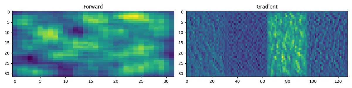To conclude, let’s see how we can chain a torch convolutional network with PyLops pylops.Smoothing2D operator. First of all, we consider a single training sample.

class Network(nn.Module):
    def __init__(self, input_channels):
        super().__init__()
        self.conv1 = nn.Conv2d(
            input_channels, input_channels // 2, kernel_size=3, padding=1
        )
        self.conv2 = nn.Conv2d(
            input_channels // 2, input_channels // 4, kernel_size=3, padding=1
        )
        self.activation = nn.LeakyReLU(0.2)
        self.maxpool = nn.MaxPool2d(kernel_size=2, stride=2)

    def forward(self, x):
        x = self.conv1(x)
        x = self.activation(x)
        x = self.conv2(x)
        x = self.activation(x)
        return x


net = Network(4)
Cop = pylops.TorchOperator(pylops.Smoothing2D((5, 5), dims=(32, 32)))

# Forward
x = torch.randn(1, 4, 32, 32).requires_grad_()
y = Cop.apply(net(x).view(-1)).reshape(32, 32)

# Backward
loss = y.sum()
loss.backward()

fig, axs = plt.subplots(1, 2, figsize=(12, 3))
axs[0].imshow(y.detach().numpy())
axs[0].set_title("Forward")
axs[0].axis("tight")
axs[1].imshow(x.grad.reshape(4 * 32, 32).T)
axs[1].set_title("Gradient")
axs[1].axis("tight")
plt.tight_layout()

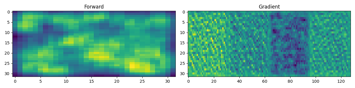
And we can do the same with a batch of 3 training samples. Note that under the hood, this effectively calls the matrix-matrix version of the forward and adjoint operator (i.e., matmat and rmatmat); for operators that do not implement these methods directly, this is simply implemented by calling the matrix-vector of the forward and adjoint operator (i.e., matvec and rmatvec)multiple times, which is less efficient.

net = Network(4)
Cop = pylops.TorchOperator(pylops.Smoothing2D((5, 5), dims=(32, 32)), batch=True)

# Forward
x = torch.randn(3, 4, 32, 32).requires_grad_()
y = Cop.apply(net(x).reshape(3, 32 * 32)).reshape(3, 32, 32)

# Backward
loss = y.sum()
loss.backward()

fig, axs = plt.subplots(1, 2, figsize=(12, 3))
axs[0].imshow(y[0].detach().numpy())
axs[0].set_title("Forward")
axs[0].axis("tight")
axs[1].imshow(x.grad[0].reshape(4 * 32, 32).T)
axs[1].set_title("Gradient")
axs[1].axis("tight")
plt.tight_layout()

Finally, whilst pylops.TorchOperator is designed such that when a PyLops linear operator is inserted into a Torch graph, the backward pass will automatically call the adjoint of the operator, it is also possible to explicitly call the forward and adjoint of the operator in the forward pass of an AD chain. This can be useful in some scenarios, for example in the implementation of so-called unrolled networks. In this case, we can simply use the forward and adjoint methods of the pylops.TorchOperator class; Torch’s AD will instead call the two methods swapped, namely adjoint and forward.

Let’s consider the following example:

\[\mathbf{y}=\textbf{A}^H (\textbf{A} \mathbf{x} - \mathbf{d})\]

whose Jacobian is given by:

\[\mathbf{J}=-\textbf{A}^H \textbf{A}\]

Let’s once again verify that the result of the product between the transposed Jacobian and a vector \(\mathbf{v}\) matches with the analytical one.

nx, ny = 10, 6
xt0 = torch.arange(nx, dtype=torch.double, requires_grad=True)
x0 = xt0.detach().numpy()
yt0 = -2 * torch.arange(ny, dtype=torch.double)
y0 = xt0.detach().numpy()

# Forward
A = np.random.normal(0.0, 1.0, (ny, nx))
At = torch.from_numpy(A)
Atop = pylops.TorchOperator(pylops.MatrixMult(A))
yt = Atop.adjoint(yt0 - Atop.forward(xt0))

# AD
v = torch.ones(nx, dtype=torch.double)
yt.backward(v, retain_graph=True)
adgrad = xt0.grad

# Analytical
JT = -At.T @ At
anagrad = torch.matmul(JT, v)

print("Input: ", x0)
print("AD gradient: ", adgrad)
print("Analytical gradient: ", anagrad)

Input:  [0. 1. 2. 3. 4. 5. 6. 7. 8. 9.]
AD gradient:  tensor([  2.8008,  -3.1352,  -1.4598,  -2.2931,  -1.8298, -10.9228,   3.4434,
         -0.7068,   2.7914,  -4.7657], dtype=torch.float64)
Analytical gradient:  tensor([  2.8008,  -3.1352,  -1.4598,  -2.2931,  -1.8298, -10.9228,   3.4434,
         -0.7068,   2.7914,  -4.7657], dtype=torch.float64)