Note
Go to the end to download the full example code.
Spread How-to
This example focuses on the pylops.basicoperators.Spread operator,
which is a highly versatile operator in PyLops to perform spreading/stacking
operations in a vectorized manner (or efficiently via Numba-jitted for loops).
The pylops.basicoperators.Spread is powerful in its generality, but
it may not be obvious for at first how to structure your code to leverage it properly.
While it is highly recommended for advanced users to inspect the
pylops.signalprocessing.Radon2D and
pylops.signalprocessing.Radon3D operators since
they are built using the pylops.basicoperators.Spread class,
here we provide a simple example on how to get started.
In this example we will recreate a simplified version of the famous linear Radon operator, which stacks data along straight lines with a given intercept and slope.
import matplotlib.pyplot as plt
import numpy as np

import pylops

plt.close("all")
Let’s first define the time and space axes as well as some auxiliary input parameters that we will use to create a Ricker wavelet
We will create a 2d data with a number of crossing linear events, to which we will
later apply our Radon transforms. We use the convenience function
pylops.utils.seismicevents.linear2d.
Let’s now define the slowness axis and use pylops.signalprocessing.Radon2D
to implement our benchmark linear Radon. Refer to the documentation of the
operator for a more detailed mathematical description of linear Radon.
Note that pxmax is in s/m, which explains the small value. Its highest value
corresponds to the lowest value of velocity in the transform. In this case we choose that
to be 1000 m/s.
Now, let’s try to reimplement this operator from scratch using pylops.basicoperators.Spread.
Using the on-the-fly approach, and we need to create a function which takes
indices of the model domain, here \((p_x, t_0)\)
where \(p_x\) is the slope and \(t_0\) is the intercept of the
parametric curve \(t(x) = t_0 + p_x x\) we wish to spread the model over
in the data domain. The function must return an array of size nx, containing
the indices corresponding to \(t(x)\).
The on-the-fly approach is useful when storing the indices in RAM may exhaust
resources, especially when computing the indices is fast. When there is
enough memory to store the full table of indices
(an array of size \(n_x \times n_t \times n_{p_x}\)) the
pylops.basicoperators.Spread operator can be used with tables instead.
We will see an example of this later.
Returning to our on-the-fly example, we need to create a function which only depends on
ipx and it0, so we create a closure around it with all our other auxiliary
variables.
def create_radon_fh(xaxis, taxis, pxaxis):
    ot = taxis[0]
    dt = taxis[1] - taxis[0]
    nt = len(taxis)

    def fh(ipx, it0):
        tx = t[it0] + xaxis * pxaxis[ipx]
        it0_frac = (tx - ot) / dt
        itx = np.rint(it0_frac)
        # Indices outside time axis set to nan
        itx[np.isin(itx, range(nt), invert=True)] = np.nan
        return itx

    return fh


fRad = create_radon_fh(x, t, px)
ROTFOp = pylops.Spread((npx, par["nt"]), (par["nx"], par["nt"]), fh=fRad)

mlinwavROTF = ROTFOp.H * mlinwav
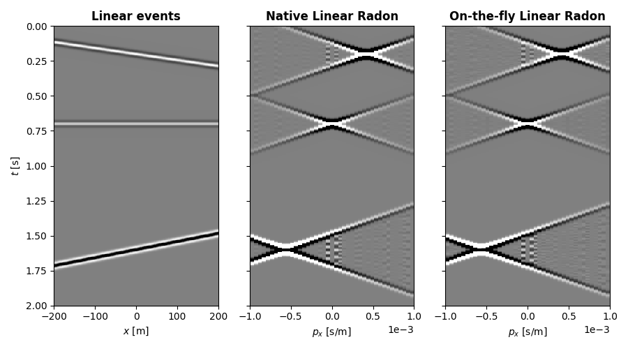
Compare the results between the native Radon transform and the one using our
on-the-fly pylops.basicoperators.Spread.
fig, axs = plt.subplots(1, 3, figsize=(9, 5), sharey=True)
axs[0].imshow(
    mlinwav.T,
    aspect="auto",
    interpolation="nearest",
    vmin=-1,
    vmax=1,
    cmap="gray",
    extent=(x.min(), x.max(), t.max(), t.min()),
)
axs[0].set_title("Linear events", fontsize=12, fontweight="bold")
axs[0].set_xlabel(r"$x$ [m]")
axs[0].set_ylabel(r"$t$ [s]")
axs[1].imshow(
    mlinwavR.T,
    aspect="auto",
    interpolation="nearest",
    vmin=-10,
    vmax=10,
    cmap="gray",
    extent=(px.min(), px.max(), t.max(), t.min()),
)
axs[1].set_title("Native Linear Radon", fontsize=12, fontweight="bold")
axs[1].set_xlabel(r"$p_x$ [s/m]")
axs[1].ticklabel_format(style="sci", axis="x", scilimits=(0, 0))

axs[2].imshow(
    mlinwavROTF.T,
    aspect="auto",
    interpolation="nearest",
    vmin=-10,
    vmax=10,
    cmap="gray",
    extent=(px.min(), px.max(), t.max(), t.min()),
)
axs[2].set_title("On-the-fly Linear Radon", fontsize=12, fontweight="bold")
axs[2].set_xlabel(r"$p_x$ [s/m]")
axs[2].ticklabel_format(style="sci", axis="x", scilimits=(0, 0))
fig.tight_layout()
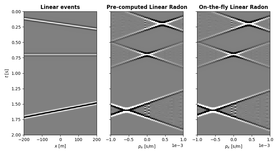
Finally, we will re-implement the example above using pre-computed tables.
This is useful when fh is expensive to compute, or requires manual edition
prior to usage.
Using a table instead of a function is simple, we just need to apply fh to
all our points and store the results.
def create_table(npx, nt, nx):
    table = np.full((npx, nt, nx), fill_value=np.nan)
    for ipx in range(npx):
        for it0 in range(nt):
            table[ipx, it0, :] = fRad(ipx, it0)
    return table


table = create_table(npx, par["nt"], par["nx"])
RPCOp = pylops.Spread((npx, par["nt"]), (par["nx"], par["nt"]), table=table)

mlinwavRPC = RPCOp.H * mlinwav
Compare the results between the pre-computed or on-the-fly Radon transforms
fig, axs = plt.subplots(1, 3, figsize=(9, 5), sharey=True)
axs[0].imshow(
    mlinwav.T,
    aspect="auto",
    interpolation="nearest",
    vmin=-1,
    vmax=1,
    cmap="gray",
    extent=(x.min(), x.max(), t.max(), t.min()),
)
axs[0].set_title("Linear events", fontsize=12, fontweight="bold")
axs[0].set_xlabel(r"$x$ [m]")
axs[0].set_ylabel(r"$t$ [s]")
axs[1].imshow(
    mlinwavRPC.T,
    aspect="auto",
    interpolation="nearest",
    vmin=-10,
    vmax=10,
    cmap="gray",
    extent=(px.min(), px.max(), t.max(), t.min()),
)
axs[1].set_title("Pre-computed Linear Radon", fontsize=12, fontweight="bold")
axs[1].set_xlabel(r"$p_x$ [s/m]")
axs[1].ticklabel_format(style="sci", axis="x", scilimits=(0, 0))

axs[2].imshow(
    mlinwavROTF.T,
    aspect="auto",
    interpolation="nearest",
    vmin=-10,
    vmax=10,
    cmap="gray",
    extent=(px.min(), px.max(), t.max(), t.min()),
)
axs[2].set_title("On-the-fly Linear Radon", fontsize=12, fontweight="bold")
axs[2].set_xlabel(r"$p_x$ [s/m]")
axs[2].ticklabel_format(style="sci", axis="x", scilimits=(0, 0))
fig.tight_layout()
Total running time of the script: (0 minutes 6.628 seconds)