Discrete Cosine Transform

This example shows how to use the pylops.signalprocessing.DCT operator. This operator performs the Discrete Cosine Transform on a (single or multi-dimensional) input array.

import matplotlib.pyplot as plt
import numpy as np

import pylops

plt.close("all")

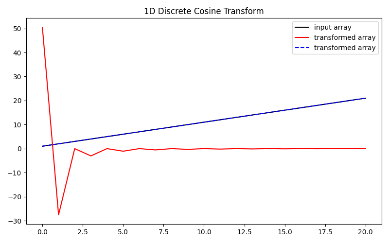
Let’s define a 1D array x of increasing numbers

n = 21
x = np.arange(n) + 1

Next we create the DCT operator with the shape of our input array as parameter, and we store the DCT coefficients in the array y. Finally, we perform the inverse using the adjoint of the operator, and we obtain the original input signal.

DOp = pylops.signalprocessing.DCT(dims=x.shape)
y = DOp @ x
xadj = DOp.H @ y

plt.figure(figsize=(8, 5))
plt.plot(x, "k", label="input array")
plt.plot(y, "r", label="transformed array")
plt.plot(xadj, "--b", label="transformed array")
plt.title("1D Discrete Cosine Transform")
plt.legend()
plt.tight_layout()

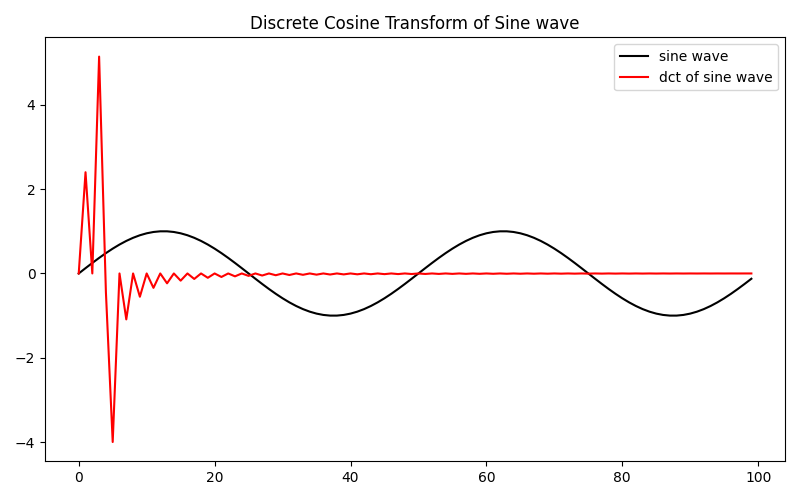
Next we apply the DCT to a sine wave

cycles = 2
resolution = 100

length = np.pi * 2 * cycles
s = np.sin(np.arange(0, length, length / resolution))
DOp = pylops.signalprocessing.DCT(dims=s.shape)
y = DOp @ s

plt.figure(figsize=(8, 5))
plt.plot(s, "k", label="sine wave")
plt.plot(y, "r", label="dct of sine wave")
plt.title("Discrete Cosine Transform of Sine wave")
plt.legend()
plt.tight_layout()

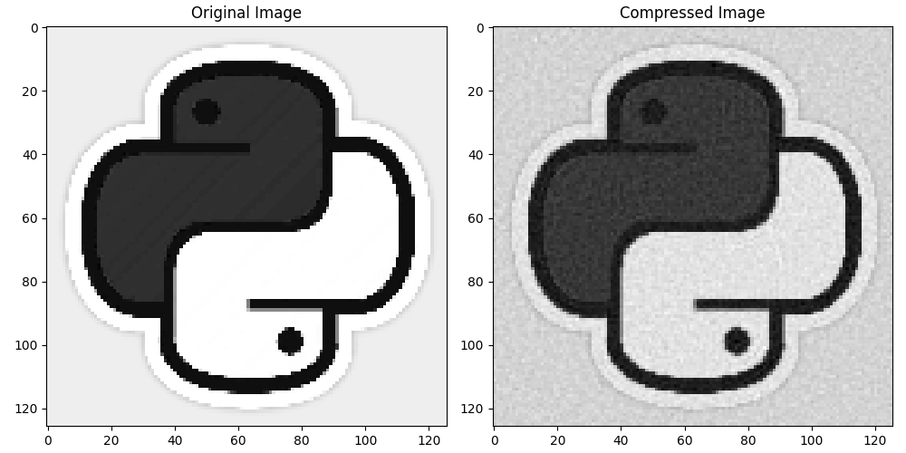
The Discrete Cosine Transform is commonly used in lossy image compression (i.e., JPEG encoding) due to its strong energy compaction nature. Here is an example of DCT being used for image compression. Note: This code is just an example and may not provide the best results for all images. You may need to adjust the threshold value to get better results.

img = np.load("../testdata/python.npy")[::5, ::5, 0]
DOp = pylops.signalprocessing.DCT(dims=img.shape)
dct_img = DOp @ img

# Set a threshold for the DCT coefficients to zero out
threshold = np.percentile(np.abs(dct_img), 70)
dct_img[np.abs(dct_img) < threshold] = 0

# Inverse DCT to get back the image
compressed_img = DOp.H @ dct_img

# Plot original and compressed images
fig, ax = plt.subplots(1, 2, figsize=(10, 5))
ax[0].imshow(img, cmap="gray")
ax[0].set_title("Original Image")
ax[1].imshow(compressed_img, cmap="gray")
ax[1].set_title("Compressed Image")
plt.tight_layout()