Synthetic seismic

This example shows how to use the pylops.utils.seismicevents module to quickly create synthetic seismic data to be used for toy examples and tests.

import matplotlib.pyplot as plt
import numpy as np

import pylops

plt.close("all")

Let’s first define the time and space axes as well as some auxiliary input parameters that we will use to create a Ricker wavelet

par = {
    "ox": -200,
    "dx": 2,
    "nx": 201,
    "oy": -100,
    "dy": 2,
    "ny": 101,
    "ot": 0,
    "dt": 0.004,
    "nt": 501,
    "f0": 20,
    "nfmax": 210,
}

# Create axis
t, t2, x, y = pylops.utils.seismicevents.makeaxis(par)

# Create wavelet
wav = pylops.utils.wavelets.ricker(np.arange(41) * par["dt"], f0=par["f0"])[0]

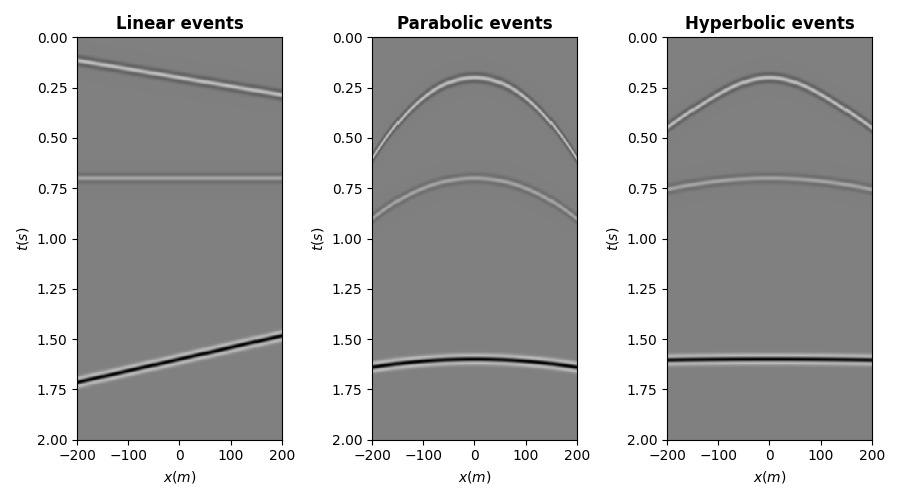
We want to create a 2d data with a number of crossing linear events using the pylops.utils.seismicevents.linear2d routine.

v = 1500
t0 = [0.2, 0.7, 1.6]
theta = [40, 0, -60]
amp = [1.0, 0.6, -2.0]

mlin, mlinwav = pylops.utils.seismicevents.linear2d(x, t, v, t0, theta, amp, wav)

We can also create a 2d data with a number of crossing parabolic events using the pylops.utils.seismicevents.parabolic2d routine.

px = [0, 0, 0]
pxx = [1e-5, 5e-6, 1e-6]

mpar, mparwav = pylops.utils.seismicevents.parabolic2d(x, t, t0, px, pxx, amp, wav)

And similarly we can create a 2d data with a number of crossing hyperbolic events using the pylops.utils.seismicevents.hyperbolic2d routine.

vrms = [500, 700, 1700]

mhyp, mhypwav = pylops.utils.seismicevents.hyperbolic2d(x, t, t0, vrms, amp, wav)

We can now visualize the different events

# sphinx_gallery_thumbnail_number = 2
fig, axs = plt.subplots(1, 3, figsize=(9, 5))
axs[0].imshow(
    mlinwav.T,
    aspect="auto",
    interpolation="nearest",
    vmin=-2,
    vmax=2,
    cmap="gray",
    extent=(x.min(), x.max(), t.max(), t.min()),
)
axs[0].set_title("Linear events", fontsize=12, fontweight="bold")
axs[0].set_xlabel(r"$x(m)$")
axs[0].set_ylabel(r"$t(s)$")
axs[1].imshow(
    mparwav.T,
    aspect="auto",
    interpolation="nearest",
    vmin=-2,
    vmax=2,
    cmap="gray",
    extent=(x.min(), x.max(), t.max(), t.min()),
)
axs[1].set_title("Parabolic events", fontsize=12, fontweight="bold")
axs[1].set_xlabel(r"$x(m)$")
axs[1].set_ylabel(r"$t(s)$")
axs[2].imshow(
    mhypwav.T,
    aspect="auto",
    interpolation="nearest",
    vmin=-2,
    vmax=2,
    cmap="gray",
    extent=(x.min(), x.max(), t.max(), t.min()),
)
axs[2].set_title("Hyperbolic events", fontsize=12, fontweight="bold")
axs[2].set_xlabel(r"$x(m)$")
axs[2].set_ylabel(r"$t(s)$")
plt.tight_layout()

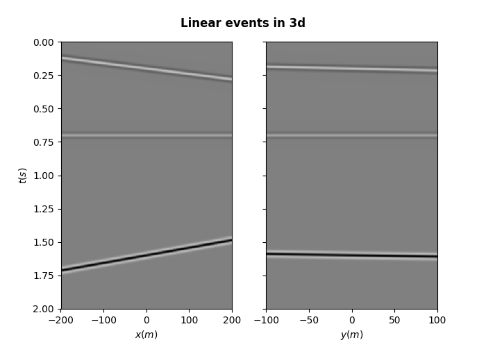
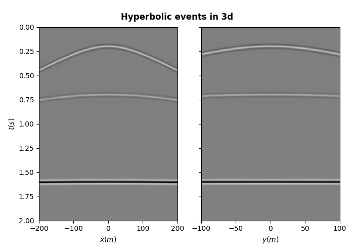
Let’s finally repeat the same exercise in 3d

phi = [20, 0, -10]
py = [0, 0, 0]
pyy = [3e-5, 1e-5, 5e-6]

mlin, mlinwav = pylops.utils.seismicevents.linear3d(
    x, y, t, v, t0, theta, phi, amp, wav
)

mpar, mparwav = pylops.utils.seismicevents.parabolic3d(
    x, y, t, t0, px, py, pxx, pyy, amp, wav
)

mhyp, mhypwav = pylops.utils.seismicevents.hyperbolic3d(
    x, y, t, t0, vrms, vrms, amp, wav
)

fig, axs = plt.subplots(1, 2, figsize=(7, 5), sharey=True)
fig.suptitle("Linear events in 3d", fontsize=12, fontweight="bold", y=0.95)
axs[0].imshow(
    mlinwav[par["ny"] // 2].T,
    aspect="auto",
    interpolation="nearest",
    vmin=-2,
    vmax=2,
    cmap="gray",
    extent=(x.min(), x.max(), t.max(), t.min()),
)
axs[0].set_xlabel(r"$x(m)$")
axs[0].set_ylabel(r"$t(s)$")
axs[1].imshow(
    mlinwav[:, par["nx"] // 2].T,
    aspect="auto",
    interpolation="nearest",
    vmin=-2,
    vmax=2,
    cmap="gray",
    extent=(y.min(), y.max(), t.max(), t.min()),
)
axs[1].set_xlabel(r"$y(m)$")

fig, axs = plt.subplots(1, 2, figsize=(7, 5), sharey=True)
fig.suptitle("Parabolic events in 3d", fontsize=12, fontweight="bold", y=0.95)
axs[0].imshow(
    mparwav[par["ny"] // 2].T,
    aspect="auto",
    interpolation="nearest",
    vmin=-2,
    vmax=2,
    cmap="gray",
    extent=(x.min(), x.max(), t.max(), t.min()),
)
axs[0].set_xlabel(r"$x(m)$")
axs[0].set_ylabel(r"$t(s)$")
axs[1].imshow(
    mparwav[:, par["nx"] // 2].T,
    aspect="auto",
    interpolation="nearest",
    vmin=-2,
    vmax=2,
    cmap="gray",
    extent=(y.min(), y.max(), t.max(), t.min()),
)
axs[1].set_xlabel(r"$y(m)$")


fig, axs = plt.subplots(1, 2, figsize=(7, 5), sharey=True)
fig.suptitle("Hyperbolic events in 3d", fontsize=12, fontweight="bold", y=0.95)
axs[0].imshow(
    mhypwav[par["ny"] // 2].T,
    aspect="auto",
    interpolation="nearest",
    vmin=-2,
    vmax=2,
    cmap="gray",
    extent=(x.min(), x.max(), t.max(), t.min()),
)
axs[0].set_xlabel(r"$x(m)$")
axs[0].set_ylabel(r"$t(s)$")
axs[1].imshow(
    mhypwav[:, par["nx"] // 2].T,
    aspect="auto",
    interpolation="nearest",
    vmin=-2,
    vmax=2,
    cmap="gray",
    extent=(y.min(), y.max(), t.max(), t.min()),
)
axs[1].set_xlabel(r"$y(m)$")
plt.tight_layout()

• 
• 
•