Non-stationary Convolution

This example shows how to use the pylops.signalprocessing.NonStationaryConvolve1D and pylops.signalprocessing.NonStationaryConvolve2D operators to perform non-stationary convolution between two signals.

Similar to their stationary counterparts, these operators can be used in the forward model of several common application in signal processing that require filtering of an input signal for a time- or space-varying instrument response.

import matplotlib.pyplot as plt
import numpy as np
from scipy.signal.windows import gaussian

import pylops
from pylops.utils.wavelets import ricker

plt.close("all")

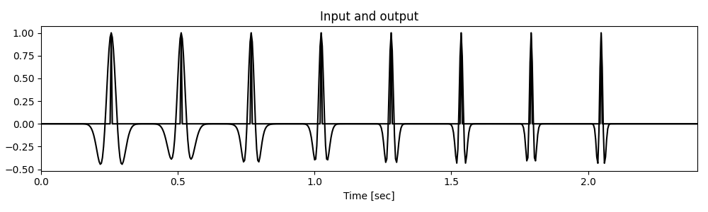
We will start by creating a zero signal of length nt and we will place a comb of unitary spikes. We also create a non-stationary filter defined by 5 equally spaced Ricker wavelets with dominant frequencies of \(f = 10, 15, 20, 25\) and \(30\) Hz.

nt = 601
dt = 0.004
t = np.arange(nt) * dt
tw = ricker(t[:51], f0=5)[1]

fs = [10, 15, 20, 25, 30]
wavs = np.stack([ricker(t[:51], f0=f)[0] for f in fs])

Cop = pylops.signalprocessing.NonStationaryConvolve1D(
    dims=nt, hs=wavs, ih=(101, 201, 301, 401, 501)
)

x = np.zeros(nt)
x[64 : nt - 64 : 64] = 1.0

y = Cop @ x

plt.figure(figsize=(10, 3))
plt.plot(t, x, "k")
plt.plot(t, y, "k")
plt.xlabel("Time [sec]")
plt.title("Input and output")
plt.xlim(0, t[-1])
plt.tight_layout()

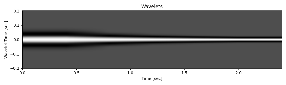
Let’s now visualize the filters in time and frequency domain

plt.figure(figsize=(10, 3))
plt.pcolormesh(t, tw, Cop.hsinterp.T, cmap="gray")
plt.xlabel("Time [sec]")
plt.ylabel("Wavelet Time [sec]")
plt.title("Wavelets")
plt.xlim(0, t[-1])
plt.tight_layout()

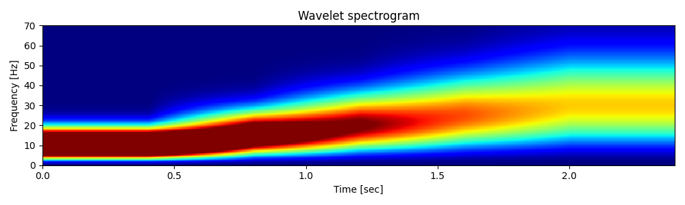
# Spectra
f = np.fft.rfftfreq(nt, dt)
Sh = np.abs(np.fft.rfft(Cop.hsinterp.T, n=nt, axis=0))

plt.figure(figsize=(10, 3))
plt.pcolormesh(t, f, Sh, cmap="jet", vmax=5e0)
plt.ylabel("Frequency [Hz]")
plt.xlabel("Time [sec]")
plt.title("Wavelet spectrogram")
plt.ylim(0, 70)
plt.xlim(0, t[-1])
plt.tight_layout()

• 
• 

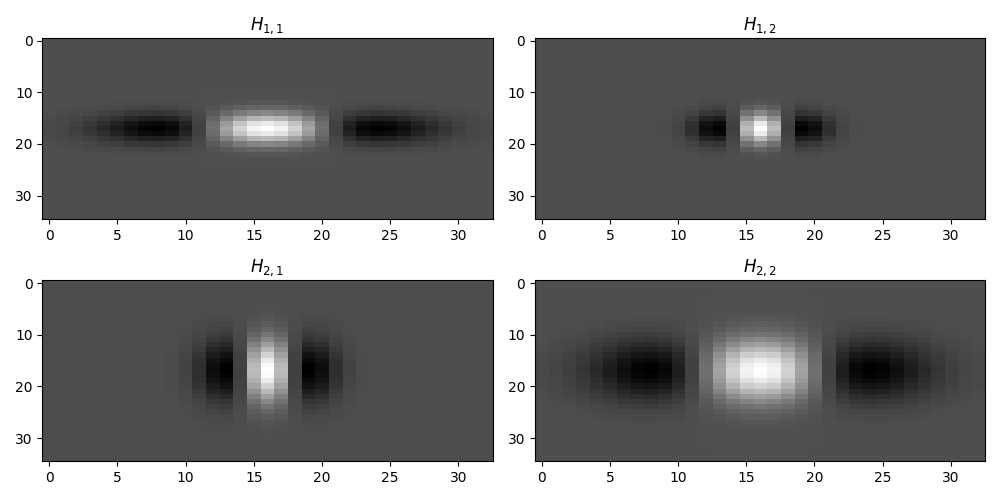
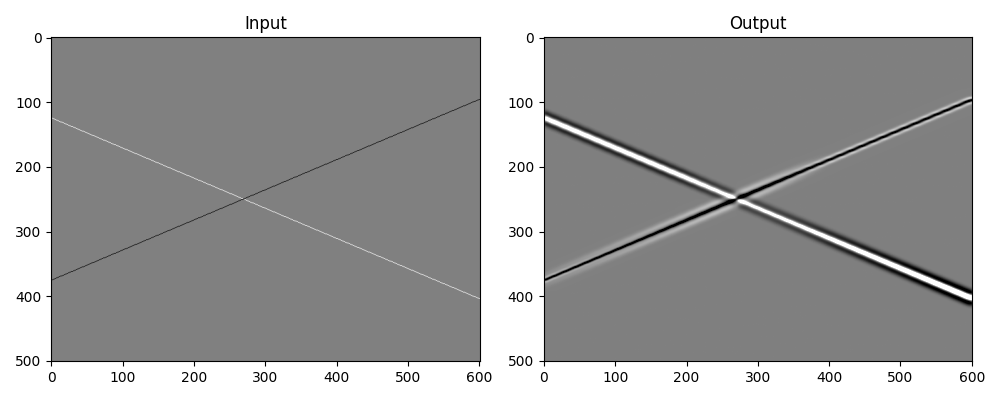
Finally, we repeat the same exercise with a 2-dimensional non-stationary filter

nx, nz = 601, 501

wav1a, _, _ = ricker(t[:17], f0=12)
wav1b, _, _ = ricker(t[:17], f0=30)
wav2a = gaussian(35, 2.0)
wav2b = gaussian(35, 4.0)

wav11 = np.outer(wav1a, wav2a[np.newaxis]).T
wav12 = np.outer(wav1b, wav2a[np.newaxis]).T
wav21 = np.outer(wav1b, wav2b[np.newaxis]).T
wav22 = np.outer(wav1a, wav2b[np.newaxis]).T
wavsize = wav11.shape

hs = np.zeros((2, 2, *wavsize))
hs[0, 0] = wav11
hs[0, 1] = wav12
hs[1, 0] = wav21
hs[1, 1] = wav22

fig, axs = plt.subplots(2, 2, figsize=(10, 5))
axs[0, 0].imshow(wav11, cmap="gray")
axs[0, 0].axis("tight")
axs[0, 0].set_title(r"$H_{1,1}$")
axs[0, 1].imshow(wav12, cmap="gray")
axs[0, 1].axis("tight")
axs[0, 1].set_title(r"$H_{1,2}$")
axs[1, 0].imshow(wav21, cmap="gray")
axs[1, 0].axis("tight")
axs[1, 0].set_title(r"$H_{2,1}$")
axs[1, 1].imshow(wav22, cmap="gray")
axs[1, 1].axis("tight")
axs[1, 1].set_title(r"$H_{2,2}$")
plt.tight_layout()

Cop = pylops.signalprocessing.NonStationaryConvolve2D(
    hs=hs, ihx=(201, 401), ihz=(201, 401), dims=(nx, nz), engine="numba"
)

x = np.zeros((nx, nz))
line1 = (np.arange(nx) * np.tan(np.deg2rad(25))).astype(int) + (nz - 1) // 4
line2 = (np.arange(nx) * np.tan(np.deg2rad(-25))).astype(int) + (3 * (nz - 1)) // 4
x[np.arange(nx), np.clip(line1, 0, nz - 1)] = 1.0
x[np.arange(nx), np.clip(line2, 0, nz - 1)] = -1.0

y = Cop @ x

fig, axs = plt.subplots(1, 2, figsize=(10, 4))
axs[0].imshow(x.T, cmap="gray", vmin=-1.0, vmax=1.0)
axs[0].axis("tight")
axs[0].set_title("Input")
axs[1].imshow(y.T, cmap="gray", vmin=-3.0, vmax=3.0)
axs[1].axis("tight")
axs[1].set_title("Output")
plt.tight_layout()

• 
•