Normal Moveout (NMO) Correction

This example shows how to create your own operator for performing normal moveout (NMO) correction to a seismic record. We will perform classic NMO using an operator created from scratch, as well as using the pylops.Spread operator.

from math import floor
from time import time

import matplotlib.pyplot as plt
import numpy as np
from mpl_toolkits.axes_grid1 import ImageGrid, make_axes_locatable
from numba import jit, prange
from scipy.interpolate import griddata
from scipy.ndimage import gaussian_filter

from pylops import LinearOperator, Spread
from pylops.utils import dottest
from pylops.utils.decorators import reshaped
from pylops.utils.seismicevents import hyperbolic2d, makeaxis
from pylops.utils.wavelets import ricker


def create_colorbar(im, ax):
    divider = make_axes_locatable(ax)
    cax = divider.append_axes("right", size="5%", pad=0.1)
    cb = fig.colorbar(im, cax=cax, orientation="vertical")
    return cax, cb

Given a common-shot or common-midpoint (CMP) record, the objective of NMO correction is to “flatten” events, that is, align events at later offsets to that of the zero offset. NMO has long been a staple of seismic data processing, used even today for initial velocity analysis and QC purposes. In addition, it can be the domain of choice for many useful processing steps, such as angle muting.

To get started, let us create a 2D seismic dataset containing some hyperbolic events representing reflections from flat reflectors. Events are created with a true RMS velocity, which we will be using as if we picked them from, for example, a semblance panel.

par = dict(ox=0, dx=40, nx=80, ot=0, dt=0.004, nt=520)
t, _, x, _ = makeaxis(par)

t0s_true = np.array([0.5, 1.22, 1.65])
vrms_true = np.array([2000.0, 2400.0, 2500.0])
amps = np.array([1, 0.2, 0.5])

freq = 10  # Hz
wav, *_ = ricker(t[:41], f0=freq)

_, data = hyperbolic2d(x, t, t0s_true, vrms_true, amp=amps, wav=wav)

# NMO correction plot
pclip = 0.5
dmax = np.max(np.abs(data))
opts = dict(
    cmap="gray_r",
    extent=[x[0], x[-1], t[-1], t[0]],
    aspect="auto",
    vmin=-pclip * dmax,
    vmax=pclip * dmax,
)

# Offset-dependent traveltime of the first hyperbolic event
t_nmo_ev1 = np.sqrt(t0s_true[0] ** 2 + (x / vrms_true[0]) ** 2)

fig, ax = plt.subplots(figsize=(4, 5))
vmax = np.max(np.abs(data))
im = ax.imshow(data.T, **opts)
ax.plot(x, t_nmo_ev1, "C1--", label="Hyperbolic moveout")
ax.plot(x, t0s_true[0] + x * 0, "C1", label="NMO-corrected")
idx = 3 * par["nx"] // 4
ax.annotate(
    "",
    xy=(x[idx], t0s_true[0]),
    xycoords="data",
    xytext=(x[idx], t_nmo_ev1[idx]),
    textcoords="data",
    fontsize=7,
    arrowprops=dict(edgecolor="w", arrowstyle="->", shrinkA=10),
)
ax.set(title="Data", xlabel="Offset [m]", ylabel="Time [s]")
cax, _ = create_colorbar(im, ax)
cax.set_ylabel("Amplitude")
ax.legend()
fig.tight_layout()

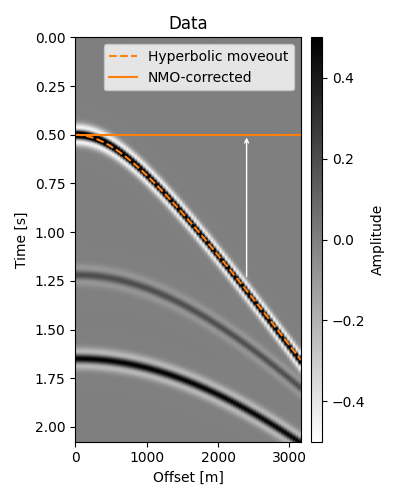
NMO correction consists of applying an offset- and time-dependent shift to each sample of the trace in such a way that all events corresponding to the same reflection will be located at the same time intercept after correction.

An arbitrary hyperbolic event at position \((t, h)\) is linked to its zero-offset traveltime \(t_0\) by the following equation

\[t(x) = \sqrt{t_0^2 + \frac{h^2}{v_\text{rms}^2(t_0)}}\]

Our strategy in applying the correction is to loop over our time axis (which we will associate to \(t_0\)) and respective RMS velocities and, for each offset, move the sample at \(t(x)\) to location \(t_0(x) \equiv t_0\). In the figure above, we are considering a single \(t_0 = 0.5\mathrm{s}\) which would have values along the dotted curve (i.e., \(t(x)\)) moved to \(t_0\) for every offset.

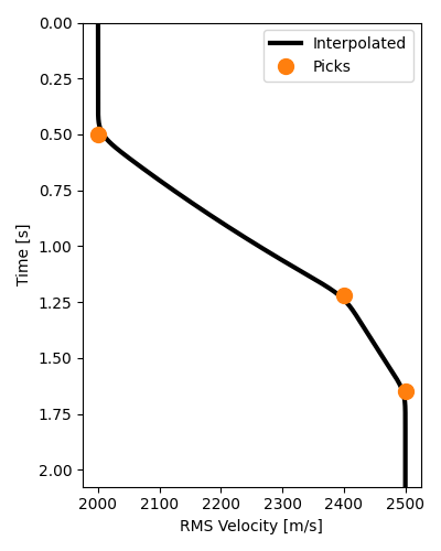
Notice that we need NMO velocities for each sample of our time axis. In this example, we actually only have 3 samples, when we need nt samples. In practice, we would have many more samples, but probably not one for each nt. To resolve this issue, we will interpolate these 3 samples to all samples of our time axis (or, more accurately, their slownesses to preserve traveltimes).

def interpolate_vrms(t0_picks, vrms_picks, taxis, smooth=None):
    assert len(t0_picks) == len(vrms_picks)

    # Sampled points in time axis
    points = np.zeros((len(t0_picks) + 2,))
    points[0] = taxis[0]
    points[-1] = taxis[-1]
    points[1:-1] = t0_picks

    # Sampled values of slowness (in s/km)
    values = np.zeros((len(vrms_picks) + 2,))
    values[0] = 1000.0 / vrms_picks[0]  # Use first slowness before t0_picks[0]
    values[-1] = 1000.0 / vrms_picks[-1]  # Use the last slowness after t0_picks[-1]
    values[1:-1] = 1000.0 / vrms_picks

    slowness = griddata(points, values, taxis, method="linear")
    if smooth is not None:
        slowness = gaussian_filter(slowness, sigma=smooth)

    return 1000.0 / slowness


vel_t = interpolate_vrms(t0s_true, vrms_true, t, smooth=11)

# Plot interpolated RMS velocities which will be used for NMO
fig, ax = plt.subplots(figsize=(4, 5))
ax.plot(vel_t, t, "k", lw=3, label="Interpolated", zorder=-1)
ax.plot(vrms_true, t0s_true, "C1o", markersize=10, label="Picks")
ax.invert_yaxis()
ax.set(xlabel="RMS Velocity [m/s]", ylabel="Time [s]", ylim=[t[-1], t[0]])
ax.legend()
fig.tight_layout()

NMO from scratch

We are very close to building our NMO correction, we just need to take care of one final issue. When moving the sample from \(t(x)\) to \(t_0\), we know that, by definition, \(t_0\) is always on our time axis grid. In contrast, \(t(x)\) may not fall exactly on a multiple of dt (our time axis sampling). Suppose its nearest sample smaller than itself (floor) is i. Instead of moving only sample i, we will be moving samples both samples i and i+1 with an appropriate weight to account for how far \(t(x)\) is from i*dt and (i+1)*dt.

@jit(nopython=True, fastmath=True, nogil=True, parallel=True)
def nmo_forward(data, taxis, haxis, vels_rms):
    dt = taxis[1] - taxis[0]
    ot = taxis[0]
    nt = len(taxis)
    nh = len(haxis)

    dnmo = np.zeros_like(data)

    # Parallel outer loop on slow axis
    for ih in prange(nh):
        h = haxis[ih]
        for it0, (t0, vrms) in enumerate(zip(taxis, vels_rms)):
            # Compute NMO traveltime
            tx = np.sqrt(t0**2 + (h / vrms) ** 2)
            it_frac = (tx - ot) / dt  # Fractional index
            it_floor = floor(it_frac)
            it_ceil = it_floor + 1
            w = it_frac - it_floor
            if 0 <= it_floor and it_ceil < nt:  # it_floor and it_ceil must be valid
                # Linear interpolation
                dnmo[ih, it0] += (1 - w) * data[ih, it_floor] + w * data[ih, it_ceil]
    return dnmo


dnmo = nmo_forward(data, t, x, vel_t)  # Compile and run

# Time execution
start = time()
nmo_forward(data, t, x, vel_t)
end = time()

print(f"Ran in {1e6*(end-start):.0f} μs")

Ran in 345 μs

# Plot Data and NMO-corrected data
fig = plt.figure(figsize=(6.5, 5))
grid = ImageGrid(
    fig,
    111,
    nrows_ncols=(1, 2),
    axes_pad=0.15,
    cbar_location="right",
    cbar_mode="single",
    cbar_size="7%",
    cbar_pad=0.15,
    aspect=False,
    share_all=True,
)
im = grid[0].imshow(data.T, **opts)
grid[0].set(title="Data", xlabel="Offset [m]", ylabel="Time [s]")
grid[0].cax.colorbar(im)
grid[0].cax.set_ylabel("Amplitude")

grid[1].imshow(dnmo.T, **opts)
grid[1].set(title="NMO-corrected Data", xlabel="Offset [m]")
plt.show()

Now that we know how to compute the forward, we’ll compute the adjoint pass. With these two functions, we can create a LinearOperator and ensure that it passes the dot-test.

@jit(nopython=True, fastmath=True, nogil=True, parallel=True)
def nmo_adjoint(dnmo, taxis, haxis, vels_rms):
    dt = taxis[1] - taxis[0]
    ot = taxis[0]
    nt = len(taxis)
    nh = len(haxis)

    data = np.zeros_like(dnmo)

    # Parallel outer loop on slow axis; use range if Numba is not installed
    for ih in prange(nh):
        h = haxis[ih]
        for it0, (t0, vrms) in enumerate(zip(taxis, vels_rms)):
            # Compute NMO traveltime
            tx = np.sqrt(t0**2 + (h / vrms) ** 2)
            it_frac = (tx - ot) / dt  # Fractional index
            it_floor = floor(it_frac)
            it_ceil = it_floor + 1
            w = it_frac - it_floor
            if 0 <= it_floor and it_ceil < nt:
                # Linear interpolation
                # In the adjoint, we must spread the same it0 to both it_floor and
                # it_ceil, since in the forward pass, both of these samples were
                # pushed onto it0
                data[ih, it_floor] += (1 - w) * dnmo[ih, it0]
                data[ih, it_ceil] += w * dnmo[ih, it0]
    return data

Finally, we can create our linear operator. To exemplify the class-based interface we will subclass pylops.LinearOperator and implement the required methods: _matvec which will compute the forward and _rmatvec which will compute the adjoint. Note the use of the reshaped decorator which allows us to pass x directly into our auxiliary function without having to do x.reshape(self.dims) and to output without having to call ravel().

class NMO(LinearOperator):
    def __init__(self, taxis, haxis, vels_rms, dtype=None):
        self.taxis = taxis
        self.haxis = haxis
        self.vels_rms = vels_rms

        dims = (len(haxis), len(taxis))
        if dtype is None:
            dtype = np.result_type(taxis.dtype, haxis.dtype, vels_rms.dtype)
        super().__init__(dims=dims, dimsd=dims, dtype=dtype)

    @reshaped
    def _matvec(self, x):
        return nmo_forward(x, self.taxis, self.haxis, self.vels_rms)

    @reshaped
    def _rmatvec(self, y):
        return nmo_adjoint(y, self.taxis, self.haxis, self.vels_rms)

With our new NMO linear operator, we can instantiate it with our current example and ensure that it passes the dot test which proves that our forward and adjoint transforms truly are adjoints of each other.

NMOOp = NMO(t, x, vel_t)
dottest(NMOOp, rtol=1e-4, verb=True)

Dot test passed, v^H(Opu)=-172.44662883153694 - u^H(Op^Hv)=-172.4466288315371

True

NMO using pylops.Spread

We learned how to implement an NMO correction and its adjoint from scratch. The adjoint has an interesting pattern, where energy taken from one domain is “spread” along a previously-defined parametric curve (the NMO hyperbola in this case). This pattern is very common in many algorithms, including Radon transform, Kirchhoff migration (also known as Total Focusing Method in ultrasonics) and many others.

For these classes of operators, PyLops offers a pylops.Spread constructor, which we will leverage to implement a version of the NMO correction. The pylops.Spread operator will take a value in the “input” domain, and spread it along a parametric curve, defined in the “output” domain. In our case, the spreading operation is the adjoint of the NMO, so our “input” domain is the NMO domain, and the “output” domain is the original data domain.

In order to use pylops.Spread, we need to define the parametric curves. This can be done through the use of a table with shape \((n_{x_i}, n_{t}, n_{x_o})\), where \(n_{x_i}\) and \(n_{t}\) represent the 2d dimensions of the “input” domain (NMO domain) and \(n_{x_o}\) and \(n_{t}\) the 2d dimensions of the “output” domain. In our NMO case, \(n_{x_i} = n_{x_o} = n_h\) represents the number of offsets. Following the documentation of pylops.Spread, the table will be used in the following manner:

d_out[ix_o, table[ix_i, it, ix_o]] += d_in[ix_i, it]

In our case, ix_o = ix_i = ih, and comparing with our NMO adjoint, it refers to \(t_0\) while table[ix, it, ix] should then provide the appropriate index for \(t(x)\). In our implementation we will also be constructing a second table containing the weights to be used for linear interpolation.

def create_tables(taxis, haxis, vels_rms):
    dt = taxis[1] - taxis[0]
    ot = taxis[0]
    nt = len(taxis)
    nh = len(haxis)

    # NaN values will be not be spread.
    # Using np.zeros has the same result but much slower.
    table = np.full((nh, nt, nh), fill_value=np.nan)
    dtable = np.full((nh, nt, nh), fill_value=np.nan)

    for ih, h in enumerate(haxis):
        for it0, (t0, vrms) in enumerate(zip(taxis, vels_rms)):
            # Compute NMO traveltime
            tx = np.sqrt(t0**2 + (h / vrms) ** 2)
            it_frac = (tx - ot) / dt
            it_floor = floor(it_frac)
            w = it_frac - it_floor
            # Both it_floor and it_floor + 1 must be valid indices for taxis
            # when using two tables (interpolation).
            if 0 <= it_floor and it_floor + 1 < nt:
                table[ih, it0, ih] = it_floor
                dtable[ih, it0, ih] = w
    return table, dtable


nmo_table, nmo_dtable = create_tables(t, x, vel_t)

SpreadNMO = Spread(
    dims=data.shape,  # "Input" shape: NMO-ed data shape
    dimsd=data.shape,  # "Output" shape: original data shape
    table=nmo_table,  # Table of time indices
    dtable=nmo_dtable,  # Table of weights for linear interpolation
    engine="numba",  # numba or numpy
).H  # To perform NMO *correction*, we need the adjoint
dottest(SpreadNMO, rtol=1e-4)

True

We see it passes the dot test, but are the results right? Let’s find out.

dnmo_spr = SpreadNMO @ data

start = time()
SpreadNMO @ data
end = time()

print(f"Ran in {1e6*(end-start):.0f} μs")

Ran in 13459 μs

Note that since v2.0, we do not need to pass a flattened array. Consequently, the output will not be flattened, but will have SpreadNMO.dimsd as shape.

# Plot Data and NMO-corrected data
fig = plt.figure(figsize=(6.5, 5))
grid = ImageGrid(
    fig,
    111,
    nrows_ncols=(1, 2),
    axes_pad=0.15,
    cbar_location="right",
    cbar_mode="single",
    cbar_size="7%",
    cbar_pad=0.15,
    aspect=False,
    share_all=True,
)
im = grid[0].imshow(data.T, **opts)
grid[0].set(title="Data", xlabel="Offset [m]", ylabel="Time [s]")
grid[0].cax.colorbar(im)
grid[0].cax.set_ylabel("Amplitude")

grid[1].imshow(dnmo_spr.T, **opts)
grid[1].set(title="NMO correction using Spread", xlabel="Offset [m]")
plt.show()

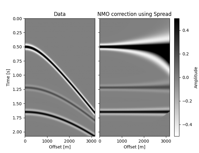
Not as blazing fast as out original implementation, but pretty good (try the “numpy” backend for comparison!). In fact, using the Spread operator for NMO will always have a speed disadvantage. While iterating over the table, it must loop over the offsets twice: one for the “input” offsets and one for the “output” offsets. We know they are the same for NMO, but since Spread is a generic operator, it does not know that. So right off the bat we can expect an 80x slowdown (nh = 80). We diminished this cost to about 30x by setting values where ix_i != ix_o to NaN, but nothing beats the custom implementation. Despite this, we can still produce the same result to numerical accuracy:

np.allclose(dnmo, dnmo_spr)

True