Multi-Dimensional Convolution

This example shows how to use the pylops.waveeqprocessing.MDC operator to convolve a 3D kernel with an input seismic data. The resulting data is a blurred version of the input data and the problem of removing such blurring is reffered to as Multi-dimensional Deconvolution (MDD) and its implementation is discussed in more details in the MDD tutorial.

import matplotlib.pyplot as plt
import numpy as np

import pylops
from pylops.utils.seismicevents import hyperbolic2d, makeaxis
from pylops.utils.tapers import taper3d
from pylops.utils.wavelets import ricker

plt.close("all")

Let’s start by creating a set of hyperbolic events to be used as our MDC kernel

# Input parameters
par = {
    "ox": -300,
    "dx": 10,
    "nx": 61,
    "oy": -500,
    "dy": 10,
    "ny": 101,
    "ot": 0,
    "dt": 0.004,
    "nt": 400,
    "f0": 20,
    "nfmax": 200,
}

t0_m = 0.2
vrms_m = 1100.0
amp_m = 1.0

t0_G = (0.2, 0.5, 0.7)
vrms_G = (1200.0, 1500.0, 2000.0)
amp_G = (1.0, 0.6, 0.5)

# Taper
tap = taper3d(par["nt"], (par["ny"], par["nx"]), (5, 5), tapertype="hanning")

# Create axis
t, t2, x, y = makeaxis(par)

# Create wavelet
wav = ricker(t[:41], f0=par["f0"])[0]

# Generate model
m, mwav = hyperbolic2d(x, t, t0_m, vrms_m, amp_m, wav)

# Generate operator
G, Gwav = np.zeros((par["ny"], par["nx"], par["nt"])), np.zeros(
    (par["ny"], par["nx"], par["nt"])
)
for iy, y0 in enumerate(y):
    G[iy], Gwav[iy] = hyperbolic2d(x - y0, t, t0_G, vrms_G, amp_G, wav)
G, Gwav = G * tap, Gwav * tap

# Add negative part to data and model
m = np.concatenate((np.zeros((par["nx"], par["nt"] - 1)), m), axis=-1)
mwav = np.concatenate((np.zeros((par["nx"], par["nt"] - 1)), mwav), axis=-1)
Gwav2 = np.concatenate((np.zeros((par["ny"], par["nx"], par["nt"] - 1)), Gwav), axis=-1)

# Define MDC linear operator
Gwav_fft = np.fft.rfft(Gwav2, 2 * par["nt"] - 1, axis=-1)
Gwav_fft = Gwav_fft[..., : par["nfmax"]]

# Move frequency/time to first axis
m, mwav = m.T, mwav.T
Gwav_fft = Gwav_fft.transpose(2, 0, 1)

# Create operator
MDCop = pylops.waveeqprocessing.MDC(
    Gwav_fft,
    nt=2 * par["nt"] - 1,
    nv=1,
    dt=0.004,
    dr=1.0,
)

# Create data
d = MDCop * m.ravel()
d = d.reshape(2 * par["nt"] - 1, par["ny"])

# Apply adjoint operator to data
madj = MDCop.H * d.ravel()
madj = madj.reshape(2 * par["nt"] - 1, par["nx"])

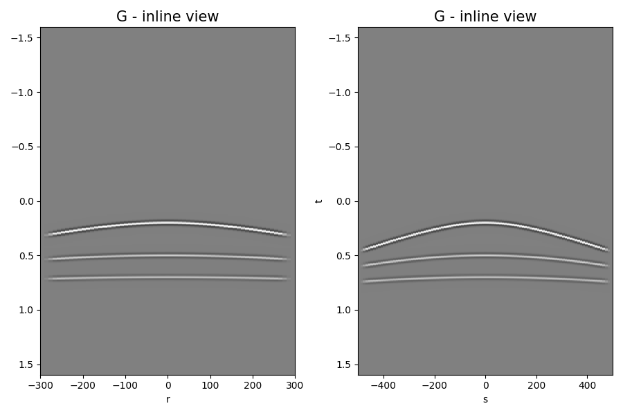
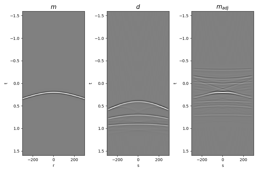
Finally let’s display the operator, input model, data and adjoint model

fig, axs = plt.subplots(1, 2, figsize=(9, 6))
axs[0].imshow(
    Gwav2[int(par["ny"] / 2)].T,
    aspect="auto",
    interpolation="nearest",
    cmap="gray",
    vmin=-Gwav2.max(),
    vmax=Gwav2.max(),
    extent=(x.min(), x.max(), t2.max(), t2.min()),
)
axs[0].set_title("G - inline view", fontsize=15)
axs[0].set_xlabel("r")
axs[1].set_ylabel("t")
axs[1].imshow(
    Gwav2[:, int(par["nx"] / 2)].T,
    aspect="auto",
    interpolation="nearest",
    cmap="gray",
    vmin=-Gwav2.max(),
    vmax=Gwav2.max(),
    extent=(y.min(), y.max(), t2.max(), t2.min()),
)
axs[1].set_title("G - inline view", fontsize=15)
axs[1].set_xlabel("s")
axs[1].set_ylabel("t")
fig.tight_layout()

fig, axs = plt.subplots(1, 3, figsize=(9, 6))
axs[0].imshow(
    mwav,
    aspect="auto",
    interpolation="nearest",
    cmap="gray",
    vmin=-mwav.max(),
    vmax=mwav.max(),
    extent=(x.min(), x.max(), t2.max(), t2.min()),
)
axs[0].set_title(r"$m$", fontsize=15)
axs[0].set_xlabel("r")
axs[0].set_ylabel("t")
axs[1].imshow(
    d,
    aspect="auto",
    interpolation="nearest",
    cmap="gray",
    vmin=-d.max(),
    vmax=d.max(),
    extent=(x.min(), x.max(), t2.max(), t2.min()),
)
axs[1].set_title(r"$d$", fontsize=15)
axs[1].set_xlabel("s")
axs[1].set_ylabel("t")
axs[2].imshow(
    madj,
    aspect="auto",
    interpolation="nearest",
    cmap="gray",
    vmin=-madj.max(),
    vmax=madj.max(),
    extent=(x.min(), x.max(), t2.max(), t2.min()),
)
axs[2].set_title(r"$m_{adj}$", fontsize=15)
axs[2].set_xlabel("s")
axs[2].set_ylabel("t")
fig.tight_layout()

• 
•