Wavelet transform

This example shows how to use the pylops.signalprocessing.DWT, pylops.signalprocessing.DWT2D, and pylops.signalprocessing.DWTND operators to perform 1-, 2-, and N-dimensional DWT. Finally, the pylops.signalprocessing.SWT2D operator is used to perform a 2-dimensional Stationary Wavelet Transform (SWT).

import matplotlib.pyplot as plt
import numpy as np

import pylops

plt.close("all")

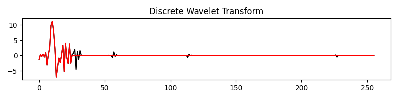
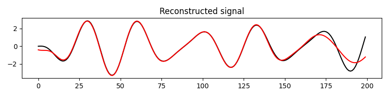
Let’s start with a 1-dimensional signal. We apply the 1-dimensional wavelet transform, keep only the first 30 coefficients and perform the inverse transform.

nt = 200
dt = 0.004
t = np.arange(nt) * dt
freqs = [10, 7, 9]
amps = [1, -2, 0.5]
x = np.sum(
    [amp * np.sin(2 * np.pi * f * t) for (f, amp) in zip(freqs, amps, strict=True)],
    axis=0,
)

Wop = pylops.signalprocessing.DWT(nt, wavelet="dmey", level=5)
y = Wop * x
yf = y.copy()
yf[25:] = 0
xinv = Wop.H * yf

plt.figure(figsize=(8, 2))
plt.plot(y, "k", label="Full")
plt.plot(yf, "r", label="Extracted")
plt.title("Discrete Wavelet Transform")
plt.tight_layout()

plt.figure(figsize=(8, 2))
plt.plot(x, "k", label="Original")
plt.plot(xinv, "r", label="Reconstructed")
plt.title("Reconstructed signal")
plt.tight_layout()

• 
• 

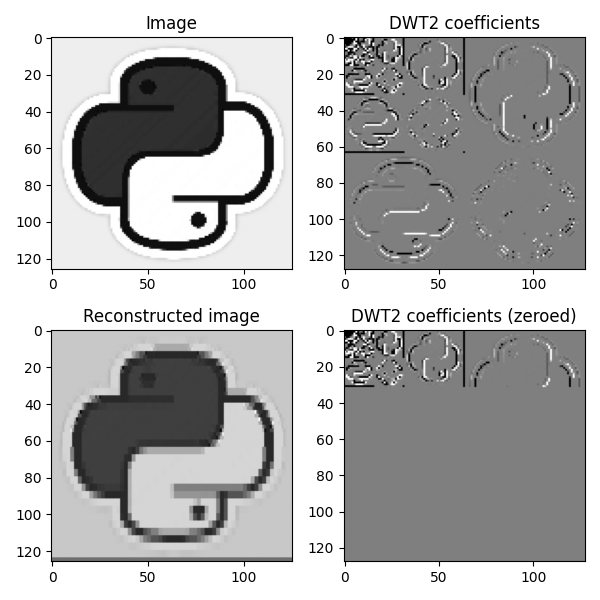
We repeat the same procedure with an image. In this case the 2-dimensional DWT will be applied instead. Only a quarter of the coefficients of the DWT will be retained in this case.

im = np.load("../testdata/python.npy")[::5, ::5, 0]

Nz, Nx = im.shape
Wop = pylops.signalprocessing.DWT2D((Nz, Nx), wavelet="haar", level=5)
y = Wop * im
yf = y.copy()
yf.flat[y.size // 4 :] = 0
iminv = Wop.H * yf

fig, axs = plt.subplots(2, 2, figsize=(6, 6))
axs[0, 0].imshow(im, cmap="gray")
axs[0, 0].set_title("Image")
axs[0, 0].axis("tight")
axs[0, 1].imshow(y, cmap="gray_r", vmin=-1e2, vmax=1e2)
axs[0, 1].set_title("DWT2 coefficients")
axs[0, 1].axis("tight")
axs[1, 0].imshow(iminv, cmap="gray")
axs[1, 0].set_title("Reconstructed image")
axs[1, 0].axis("tight")
axs[1, 1].imshow(yf, cmap="gray_r", vmin=-1e2, vmax=1e2)
axs[1, 1].set_title("DWT2 coefficients (zeroed)")
axs[1, 1].axis("tight")
plt.tight_layout()

Let us now try the same with a 3D volumetric model, where we use the N-dimensional DWT. This time, we only retain 10 percent of the coefficients of the DWT.

nx = 128
ny = 256
nz = 128

x = np.arange(nx)
y = np.arange(ny)
z = np.arange(nz)

xx, yy, zz = np.meshgrid(x, y, z, indexing="ij")
# Generate a 3D model with two block anomalies
m = np.ones_like(xx, dtype=float)
block1 = (xx > 10) & (xx < 60) & (yy > 100) & (yy < 150) & (zz > 20) & (zz < 70)
block2 = (xx > 70) & (xx < 80) & (yy > 100) & (yy < 200) & (zz > 10) & (zz < 50)
m[block1] = 1.2
m[block2] = 0.8
Wop = pylops.signalprocessing.DWTND((nx, ny, nz), wavelet="haar", level=3)
y = Wop * m

ratio = 0.1
yf = y.copy()
yf.flat[int(ratio * y.size) :] = 0
iminv = Wop.H * yf

fig, axs = plt.subplots(2, 2, figsize=(6, 6))
axs[0, 0].imshow(m[:, :, 30], cmap="gray")
axs[0, 0].set_title("Model (Slice at z=30)")
axs[0, 0].axis("tight")
axs[0, 1].imshow(y[:, :, 90], cmap="gray_r")
axs[0, 1].set_title("DWTNT coefficients")
axs[0, 1].axis("tight")
axs[1, 0].imshow(iminv[:, :, 30], cmap="gray")
axs[1, 0].set_title("Reconstructed model (Slice at z=30)")
axs[1, 0].axis("tight")
axs[1, 1].imshow(yf[:, :, 90], cmap="gray_r")
axs[1, 1].set_title("DWTNT coefficients (zeroed)")
axs[1, 1].axis("tight")
plt.tight_layout()

Finally, we consider the Stationary Wavelet Transform (SWT). Contrarily to the DWT, the SWT does not decimate the coefficients at each level, making it shift-invariant at the cost of redundancy (the number of coefficients is larger than the number of samples in the input). The coefficients of the SWT are stacked along a new leading axis, starting with the approximation coefficients at the coarsest level followed by the horizontal, vertical, and diagonal details of each level (from the coarsest to the finest).

Nz, Nx = im.shape
SWTop = pylops.signalprocessing.SWT2D((Nz, Nx), wavelet="haar", level=3)
ys = SWTop * im

fig, axs = plt.subplots(1, 4, figsize=(12, 3))
for iax, (ax, title) in enumerate(zip(axs, ["cA3", "cH3", "cV3", "cD3"], strict=True)):
    ax.imshow(ys[iax], cmap="gray" if iax == 0 else "gray_r")
    ax.set_title(title)
    ax.axis("tight")
plt.tight_layout()