20. Image Domain Least-squares migration

Seismic migration is the process by which seismic data are manipulated to create an image of the subsurface reflectivity.

In one of the previous tutorials, we have seen how the process can be formulated as an inverse problem, which requires access to a demigration-migration engine. As performing repeated migrations and demigrations can be very expensive, an alternative approach to obtain accurate and high-resolution estimate of the subsurface reflectivity has emerged under the name of image-domain least-squares migration.

In image-domain least-squares migration, we identify a direct, linear link between the migrated image \(\mathbf{m}\) and the sought after reflectivity \(\mathbf{r}\), namely:

\[\mathbf{m} = \mathbf{H} \mathbf{r}\]

Here \(\mathbf{H}\) is the Hessian, which can be written as:

\[\mathbf{H} = \mathbf{L}^H \mathbf{L}\]

where \(\mathbf{L}\) is the demigration operator, whilst its adjoint \(\mathbf{L}^H\) is the migration operator. In other words, we say that the migrated image can be seen as the result of a pair of demigration/migration of the reflectivity.

Whilst there exists different ways to estimate \(\mathbf{H}\), the approach that we will be using here entails applying demigration and migration to a special reflectivity model composed of regularly space scatterers. What we obtain is the spatially-varying impulse response of the migration operator, where each filter is also usually referred to as local point spread function (PSF).

Once these PSFs are computed (an operation that requires one migration and one demigration, much cheaper than what we do in LSM), the migrated image can be deconvolved using the pylops.signalprocessing.NonStationaryConvolve2D operator.

import matplotlib.pyplot as plt
import numpy as np

import pylops

plt.close("all")
np.random.seed(0)

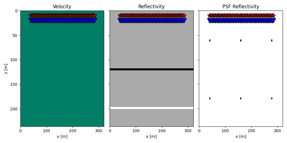
To start we create a simple model with 2 interfaces (the same we used in the LSM tutorial) and our PSF model with regularly spaced scatteres

# Velocity Model
nx, nz = 81, 60
dx, dz = 4, 4
x, z = np.arange(nx) * dx, np.arange(nz) * dz
v0 = 1000  # initial velocity
kv = 0.0  # gradient
vel = np.outer(np.ones(nx), v0 + kv * z)

# Reflectivity Model
refl = np.zeros((nx, nz))
refl[:, 30] = -1
refl[:, 50] = 0.5

# PSF Reflectivity Model
psfrefl = np.zeros((nx, nz))
psfin = (10, 15)
psfend = (-10, -5)
psfj = (30, 30)

psfx = np.arange(psfin[0], nx + psfend[0], psfj[0])
psfz = np.arange(psfin[1], nz + psfend[1], psfj[1])
Psfx, Psfz = np.meshgrid(psfx, psfz, indexing="ij")
psfrefl[psfin[0] : psfend[0] : psfj[0], psfin[1] : psfend[-1] : psfj[-1]] = 1

# Receivers
nr = 51
rx = np.linspace(10 * dx, (nx - 10) * dx, nr)
rz = 20 * np.ones(nr)
recs = np.vstack((rx, rz))
dr = recs[0, 1] - recs[0, 0]

# Sources
ns = 51
sx = np.linspace(dx * 10, (nx - 10) * dx, ns)
sz = 10 * np.ones(ns)
sources = np.vstack((sx, sz))
ds = sources[0, 1] - sources[0, 0]

fig, axs = plt.subplots(1, 3, sharey=True, figsize=(10, 5))
axs[0].imshow(vel.T, cmap="summer", extent=(x[0], x[-1], z[-1], z[0]))
axs[0].scatter(recs[0], recs[1], marker="v", s=150, c="b", edgecolors="k")
axs[0].scatter(sources[0], sources[1], marker="*", s=150, c="r", edgecolors="k")
axs[0].axis("tight")
axs[0].set_xlabel("x [m]"), axs[0].set_ylabel("z [m]")
axs[0].set_title("Velocity")
axs[0].set_xlim(x[0], x[-1])

axs[1].imshow(refl.T, cmap="gray", extent=(x[0], x[-1], z[-1], z[0]))
axs[1].scatter(recs[0], recs[1], marker="v", s=150, c="b", edgecolors="k")
axs[1].scatter(sources[0], sources[1], marker="*", s=150, c="r", edgecolors="k")
axs[1].axis("tight")
axs[1].set_xlabel("x [m]")
axs[1].set_title("Reflectivity")
axs[1].set_xlim(x[0], x[-1])

axs[2].imshow(psfrefl.T, cmap="gray_r", extent=(x[0], x[-1], z[-1], z[0]))
axs[2].scatter(recs[0], recs[1], marker="v", s=150, c="b", edgecolors="k")
axs[2].scatter(sources[0], sources[1], marker="*", s=150, c="r", edgecolors="k")
axs[2].axis("tight")
axs[2].set_xlabel("x [m]")
axs[2].set_title("PSF Reflectivity")
axs[2].set_xlim(x[0], x[-1])
plt.tight_layout()

We can now create our Kirchhoff modelling object which we will use to model and migrate the data, as well as to model and migrate the PSF model.

nt = 151
dt = 0.004
t = np.arange(nt) * dt
wav, wavt, wavc = pylops.utils.wavelets.ricker(t[:41], f0=20)

kop = pylops.waveeqprocessing.Kirchhoff(
    z,
    x,
    t,
    sources,
    recs,
    v0,
    wav,
    wavc,
    mode="analytic",
    dynamic=False,
    wavfilter=True,
    engine="numba",
)
kopdyn = pylops.waveeqprocessing.Kirchhoff(
    z,
    x,
    t,
    sources,
    recs,
    v0,
    wav,
    wavc,
    mode="analytic",
    dynamic=True,
    wavfilter=True,
    aperture=2,
    angleaperture=50,
    engine="numba",
)

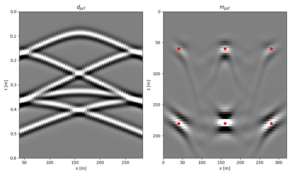
d = kop @ refl
mmig = kopdyn.H @ d

dpsf = kop @ psfrefl
mmigpsf = kopdyn.H @ dpsf

fig, axs = plt.subplots(1, 2, figsize=(10, 6))
axs[0].imshow(
    dpsf[ns // 2, :, :].T,
    extent=(rx[0], rx[-1], t[-1], t[0]),
    cmap="gray",
    vmin=-200,
    vmax=200,
)
axs[0].axis("tight")
axs[0].set_xlabel("x [m]"), axs[0].set_ylabel("t [m]")
axs[0].set_title(r"$d_{psf}$")
axs[1].imshow(
    mmigpsf.T, cmap="gray", extent=(x[0], x[-1], z[-1], z[0]), vmin=-200, vmax=200
)
axs[1].scatter(Psfx.ravel() * dx, Psfz.ravel() * dz, c="r")
axs[1].set_xlabel("x [m]"), axs[1].set_ylabel("z [m]")
axs[1].set_title(r"$m_{psf}$")
axs[1].axis("tight")
plt.tight_layout()

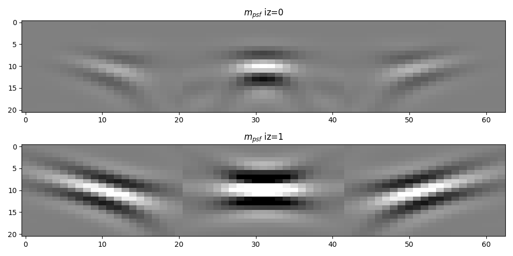
We can now extract the local PSFs and create the 2-dimensional non-stationary filtering operator

psfsize = (21, 21)
psfs = np.zeros((len(psfx), len(psfz), *psfsize))

for ipx, px in enumerate(psfx):
    for ipz, pz in enumerate(psfz):
        psfs[ipx, ipz] = mmigpsf[
            int(px - psfsize[0] // 2) : int(px + psfsize[0] // 2 + 1),
            int(pz - psfsize[1] // 2) : int(pz + psfsize[1] // 2 + 1),
        ]

fig, axs = plt.subplots(2, 1, figsize=(10, 5))
axs[0].imshow(
    psfs[:, 0].reshape(len(psfx) * psfsize[0], psfsize[1]).T,
    cmap="gray",
    vmin=-200,
    vmax=200,
)
axs[0].set_title(r"$m_{psf}$ iz=0")
axs[0].axis("tight")
axs[1].imshow(
    psfs[:, 1].reshape(len(psfx) * psfsize[0], psfsize[1]).T,
    cmap="gray",
    vmin=-200,
    vmax=200,
)
axs[1].set_title(r"$m_{psf}$ iz=1")
axs[1].axis("tight")
plt.tight_layout()

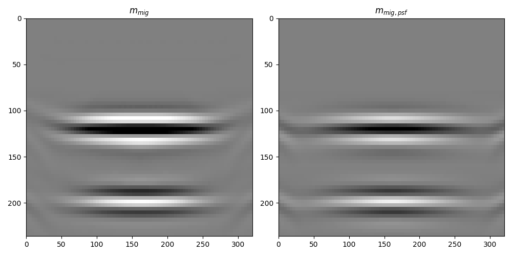
Cop = pylops.signalprocessing.NonStationaryConvolve2D(
    hs=psfs, ihx=psfx, ihz=psfz, dims=(nx, nz), engine="numba"
)

mmigpsf = Cop @ refl

fig, axs = plt.subplots(1, 2, figsize=(10, 5))
axs[0].imshow(
    mmig.T, cmap="gray", extent=(x[0], x[-1], z[-1], z[0]), vmin=-1e3, vmax=1e3
)
axs[0].set_title(r"$m_{mig}$")
axs[0].axis("tight")
axs[1].imshow(
    mmigpsf.T, cmap="gray", extent=(x[0], x[-1], z[-1], z[0]), vmin=-1e3, vmax=1e3
)
axs[1].set_title(r"$m_{mig, psf}$")
axs[1].axis("tight")
plt.tight_layout()

• 
• 

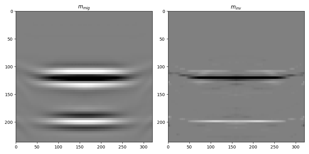
Finally, we are ready to invert our seismic image for its corresponding reflectivity using the pylops.optimization.sparsity.fista solver.

minv, _, resnorm = pylops.optimization.sparsity.fista(
    Cop, mmig.ravel(), eps=1e5, niter=100, eigsdict=dict(niter=5, tol=1e-2), show=True
)
minv = minv.reshape(nx, nz)

fig, axs = plt.subplots(1, 2, figsize=(10, 5))
axs[0].imshow(
    mmig.T, cmap="gray", extent=(x[0], x[-1], z[-1], z[0]), vmin=-500, vmax=500
)
axs[0].set_title(r"$m_{mig}$")
axs[0].axis("tight")
axs[1].imshow(minv.T, cmap="gray", extent=(x[0], x[-1], z[-1], z[0]), vmin=-1, vmax=1)
axs[1].set_title(r"$m_{inv}$")
axs[1].axis("tight")
plt.tight_layout()

FISTA (soft thresholding)
--------------------------------------------------------------------------------
The Operator Op has 4860 rows and 4860 cols
eps = 1.000000e+05      tol = 1.000000e-10      niter = 100
alpha = 1.022879e-05    thresh = 5.114397e-01
--------------------------------------------------------------------------------
   Itn          x[0]              r2norm     r12norm     xupdate
     1      -0.0000e+00         4.220e+05   4.220e+05   0.000e+00

Iterations = 1        Total time (s) = 0.32
--------------------------------------------------------------------------------

For a more advanced set of examples of both reflectivity and impedance image-domain LSM head over to this notebook.