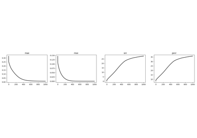
pylops.optimization.cls_sparsity.ISTA#
- class pylops.optimization.cls_sparsity.ISTA(Op, callbacks=None)[source]#
Iterative Shrinkage-Thresholding Algorithm (ISTA).
Solve an optimization problem with \(L_p, \; p=0, 0.5, 1\) regularization, given the operator
Opand datay. The operator can be real or complex, and should ideally be either square \(N=M\) or underdetermined \(N<M\).- Parameters
- Op
pylops.LinearOperator Operator to invert
- Op
- Raises
- NotImplementedError
If
threshkindis different from hard, soft, half, soft-percentile, or half-percentile- ValueError
If
perc=Nonewhenthreshkindis soft-percentile or half-percentile- ValueError
If
monitorres=Trueand residual increases
See also
OMPOrthogonal Matching Pursuit (OMP).
FISTAFast Iterative Shrinkage-Thresholding Algorithm (FISTA).
SPGL1Spectral Projected-Gradient for L1 norm (SPGL1).
SplitBregmanSplit Bregman for mixed L2-L1 norms.
Notes
Solves the following synthesis problem for the operator \(\mathbf{Op}\) and the data \(\mathbf{y}\):
\[J = \|\mathbf{y} - \mathbf{Op}\,\mathbf{x}\|_2^2 + \epsilon \|\mathbf{x}\|_p\]or the analysis problem:
\[J = \|\mathbf{y} - \mathbf{Op}\,\mathbf{x}\|_2^2 + \epsilon \|\mathbf{SOp}^H\,\mathbf{x}\|_p\]if
SOpis provided. Note that in the first case,SOpshould be assimilated in the modelling operator (i.e.,Op=GOp * SOp).The Iterative Shrinkage-Thresholding Algorithms (ISTA) [1] is used, where \(p=0, 0.5, 1\). This is a very simple iterative algorithm which applies the following step:
\[\mathbf{x}^{(i+1)} = T_{(\epsilon \alpha /2, p)} \left(\mathbf{x}^{(i)} + \alpha\,\mathbf{Op}^H \left(\mathbf{y} - \mathbf{Op}\,\mathbf{x}^{(i)}\right)\right)\]or
\[\mathbf{x}^{(i+1)} = \mathbf{SOp}\,\left\{T_{(\epsilon \alpha /2, p)} \mathbf{SOp}^H\,\left(\mathbf{x}^{(i)} + \alpha\,\mathbf{Op}^H \left(\mathbf{y} - \mathbf{Op} \,\mathbf{x}^{(i)}\right)\right)\right\}\]where \(\epsilon \alpha /2\) is the threshold and \(T_{(\tau, p)}\) is the thresholding rule. The most common variant of ISTA uses the so-called soft-thresholding rule \(T(\tau, p=1)\). Alternatively an hard-thresholding rule is used in the case of \(p=0\) or a half-thresholding rule is used in the case of \(p=1/2\). Finally, percentile bases thresholds are also implemented: the damping factor is not used anymore an the threshold changes at every iteration based on the computed percentile.
- 1
Daubechies, I., Defrise, M., and De Mol, C., “An iterative thresholding algorithm for linear inverse problems with a sparsity constraint”, Communications on pure and applied mathematics, vol. 57, pp. 1413-1457. 2004.
Methods
__init__(Op[, callbacks])callback(x, *args, **kwargs)Callback routine
finalize([show])Finalize solver
run(x[, niter, show, itershow])Run solver
setup(y[, x0, niter, SOp, eps, alpha, ...])Setup solver
solve(y[, x0, niter, SOp, eps, alpha, ...])Run entire solver
step(x[, show])Run one step of solver

