Note
Go to the end to download the full example code.
1D, 2D and 3D Sliding
This example shows how to use the
pylops.signalprocessing.Sliding1D,
pylops.signalprocessing.Sliding2D
and pylops.signalprocessing.Sliding3D operators
to perform repeated transforms over small strides of a 1-, 2- or 3-dimensional
array.
For the 1-d case, the transform that we apply in this example is the
pylops.signalprocessing.FFT.
For the 2- and 3-d cases, the transform that we apply in this example is the
pylops.signalprocessing.Radon2D
(and pylops.signalprocessing.Radon3D) but this operator has been
design to allow a variety of transforms as long as they operate with signals
that are 2 or 3-dimensional in nature, respectively.
import matplotlib.pyplot as plt
import numpy as np

import pylops

plt.close("all")
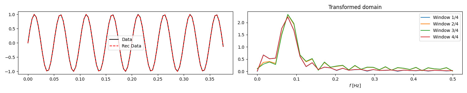
Let’s start by creating a 1-dimensional array of size \(n_t\) and create a sliding operator to compute its transformed representation.
# sliding window parameters
nwin = 26
nover = 3
nop = 64

# length of input signal (chosen to ensure perfect match with sliding windows)
dimd = 95
t = np.arange(dimd) * 0.004
data = np.sin(2 * np.pi * 20 * t)

Op = pylops.signalprocessing.FFT(nwin, nfft=nop, real=True)

nwins, dim, mwin_inends, dwin_inends = pylops.signalprocessing.sliding1d_design(
    dimd, nwin, nover, (nop + 2) // 2
)
Slid = pylops.signalprocessing.Sliding1D(
    Op.H,
    dim,
    dimd,
    nwin,
    nover,
    tapertype=None,
)

x = Slid.H * data
We now create a similar operator but we also add a taper to the overlapping
parts of the patches and use it to reconstruct the original signal.
This is done by simply using the adjoint of the
pylops.signalprocessing.Sliding1D operator. Note that for non-
orthogonal operators, this must be replaced by an inverse.
Slid = pylops.signalprocessing.Sliding1D(
    Op.H, dim, dimd, nwin, nover, tapertype="cosine"
)

reconstructed_data = Slid * x

fig, axs = plt.subplots(1, 2, figsize=(15, 3))
axs[0].plot(t, data, "k", label="Data")
axs[0].plot(t, reconstructed_data.real, "--r", label="Rec Data")
axs[0].legend()
axs[1].set(xlabel=r"$t$ [s]", title="Original domain")
for i in range(nwins):
    axs[1].plot(Op.f, np.abs(x[i, :]), label=f"Window {i+1}/{nwins}")
axs[1].set(xlabel=r"$f$ [Hz]", title="Transformed domain")
axs[1].legend()
plt.tight_layout()
We now create a 2-dimensional array of size \(n_x \times n_t\) composed of 3 parabolic events
par = {"ox": -140, "dx": 2, "nx": 140, "ot": 0, "dt": 0.004, "nt": 200, "f0": 20}

v = 1500
t0 = [0.2, 0.4, 0.5]
px = [0, 0, 0]
pxx = [1e-5, 5e-6, 1e-20]
amp = [1.0, -2, 0.5]

# Create axis
t, t2, x, y = pylops.utils.seismicevents.makeaxis(par)

# Create wavelet
wav = pylops.utils.wavelets.ricker(t[:41], f0=par["f0"])[0]

# Generate model
_, data = pylops.utils.seismicevents.parabolic2d(x, t, t0, px, pxx, amp, wav)
We want to divide this 2-dimensional data into small overlapping
patches in the spatial direction and apply the adjoint of the
pylops.signalprocessing.Radon2D operator to each patch. This is
done by simply using the adjoint of the
pylops.signalprocessing.Sliding2D operator
winsize = 36
overlap = 10
npx = 61
px = np.linspace(-5e-3, 5e-3, npx)
dimsd = data.shape

# Sliding window transform without taper
Op = pylops.signalprocessing.Radon2D(
    t,
    np.linspace(-par["dx"] * winsize // 2, par["dx"] * winsize // 2, winsize),
    px,
    centeredh=True,
    kind="linear",
    engine="numba",
)

nwins, dims, mwin_inends, dwin_inends = pylops.signalprocessing.sliding2d_design(
    dimsd, winsize, overlap, (npx, par["nt"])
)
Slid = pylops.signalprocessing.Sliding2D(
    Op, dims, dimsd, winsize, overlap, tapertype=None
)

radon = Slid.H * data
We now create a similar operator but we also add a taper to the overlapping parts of the patches.
Slid = pylops.signalprocessing.Sliding2D(
    Op, dims, dimsd, winsize, overlap, tapertype="cosine"
)
reconstructed_data = Slid * radon

# Reshape for plotting
radon = radon.reshape(dims)
reconstructed_data = reconstructed_data.reshape(dimsd)
We will see that our reconstructed signal presents some small artifacts. This is because we have not inverted our operator but simply applied the adjoint to estimate the representation of the input data in the Radon domain. We can do better if we use the inverse instead.
radoninv = Slid.div(data.ravel(), niter=10)
reconstructed_datainv = Slid * radoninv.ravel()

radoninv = radoninv.reshape(dims)
reconstructed_datainv = reconstructed_datainv.reshape(dimsd)
Let’s finally visualize all the intermediate results as well as our final
data reconstruction after inverting the
pylops.signalprocessing.Sliding2D operator.
fig, axs = plt.subplots(2, 3, sharey=True, figsize=(12, 10))
im = axs[0][0].imshow(data.T, cmap="gray")
axs[0][0].set_title("Original data")
plt.colorbar(im, ax=axs[0][0])
axs[0][0].axis("tight")
im = axs[0][1].imshow(radon.T, cmap="gray")
axs[0][1].set_title("Adjoint Radon")
plt.colorbar(im, ax=axs[0][1])
axs[0][1].axis("tight")
im = axs[0][2].imshow(reconstructed_data.T, cmap="gray")
axs[0][2].set_title("Reconstruction from adjoint")
plt.colorbar(im, ax=axs[0][2])
axs[0][2].axis("tight")
axs[1][0].axis("off")
im = axs[1][1].imshow(radoninv.T, cmap="gray")
axs[1][1].set_title("Inverse Radon")
plt.colorbar(im, ax=axs[1][1])
axs[1][1].axis("tight")
im = axs[1][2].imshow(reconstructed_datainv.T, cmap="gray")
axs[1][2].set_title("Reconstruction from inverse")
plt.colorbar(im, ax=axs[1][2])
axs[1][2].axis("tight")

for i in range(0, 114, 24):
    axs[0][0].axvline(i, color="w", lw=1, ls="--")
    axs[0][0].axvline(i + winsize, color="k", lw=1, ls="--")
    axs[0][0].text(
        i + winsize // 2,
        par["nt"] - 10,
        "w" + str(i // 24),
        ha="center",
        va="center",
        weight="bold",
        color="w",
    )

for i in range(0, 305, 61):
    axs[0][1].axvline(i, color="w", lw=1, ls="--")
    axs[0][1].text(
        i + npx // 2,
        par["nt"] - 10,
        "w" + str(i // 61),
        ha="center",
        va="center",
        weight="bold",
        color="w",
    )
    axs[1][1].axvline(i, color="w", lw=1, ls="--")
    axs[1][1].text(
        i + npx // 2,
        par["nt"] - 10,
        "w" + str(i // 61),
        ha="center",
        va="center",
        weight="bold",
        color="w",
    )
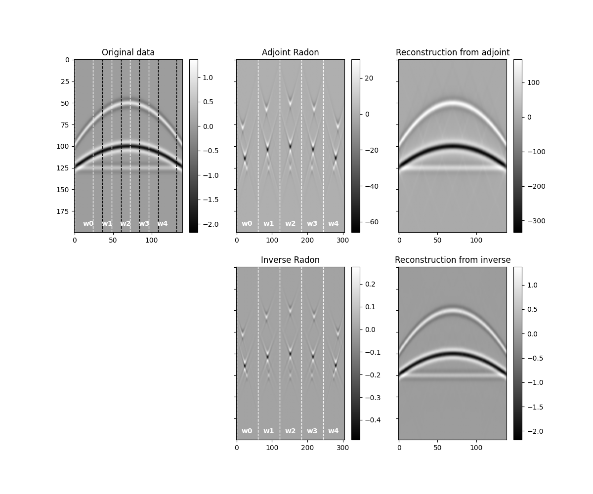
We notice two things, i)provided small enough patches and a transform that can explain data locally, we have been able reconstruct our original data almost to perfection. ii) inverse is betten than adjoint as expected as the adjoin does not only introduce small artifacts but also does not respect the original amplitudes of the data.
An appropriate transform alongside with a sliding window approach will result a very good approach for interpolation (or regularization) or irregularly sampled seismic data.
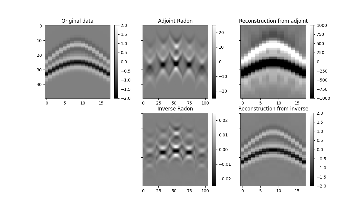
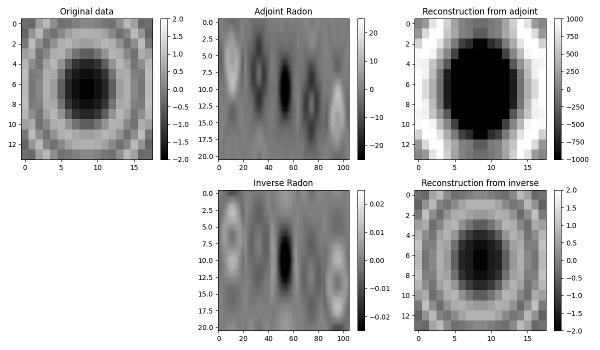
Finally we do the same for a 3-dimensional array of size \(n_y \times n_x \times n_t\) composed of 3 hyperbolic events
par = {
    "oy": -13,
    "dy": 2,
    "ny": 14,
    "ox": -17,
    "dx": 2,
    "nx": 18,
    "ot": 0,
    "dt": 0.004,
    "nt": 50,
    "f0": 30,
}

vrms = [200, 200]
t0 = [0.05, 0.1]
amp = [1.0, -2]

# Create axis
t, t2, x, y = pylops.utils.seismicevents.makeaxis(par)

# Create wavelet
wav = pylops.utils.wavelets.ricker(t[:41], f0=par["f0"])[0]

# Generate model
_, data = pylops.utils.seismicevents.hyperbolic3d(x, y, t, t0, vrms, vrms, amp, wav)

# Sliding window plan
winsize = (5, 6)
overlap = (2, 3)
npx = 21
px = np.linspace(-5e-3, 5e-3, npx)
dimsd = data.shape

# Sliding window transform without taper
Op = pylops.signalprocessing.Radon3D(
    t,
    np.linspace(-par["dy"] * winsize[0] // 2, par["dy"] * winsize[0] // 2, winsize[0]),
    np.linspace(-par["dx"] * winsize[1] // 2, par["dx"] * winsize[1] // 2, winsize[1]),
    px,
    px,
    centeredh=True,
    kind="linear",
    engine="numba",
)

nwins, dims, mwin_inends, dwin_inends = pylops.signalprocessing.sliding3d_design(
    dimsd, winsize, overlap, (npx, npx, par["nt"])
)
Slid = pylops.signalprocessing.Sliding3D(
    Op, dims, dimsd, winsize, overlap, (npx, npx), tapertype=None
)

radon = Slid.H * data

Slid = pylops.signalprocessing.Sliding3D(
    Op, dims, dimsd, winsize, overlap, (npx, npx), tapertype="cosine"
)

reconstructed_data = Slid * radon

radoninv = Slid.div(data.ravel(), niter=10)
radoninv = radoninv.reshape(Slid.dims)
reconstructed_datainv = Slid * radoninv

fig, axs = plt.subplots(2, 3, sharey=True, figsize=(12, 7))
im = axs[0][0].imshow(data[par["ny"] // 2].T, cmap="gray", vmin=-2, vmax=2)
axs[0][0].set_title("Original data")
plt.colorbar(im, ax=axs[0][0])
axs[0][0].axis("tight")
im = axs[0][1].imshow(
    radon[nwins[0] // 2, :, :, npx // 2].reshape(nwins[1] * npx, par["nt"]).T,
    cmap="gray",
    vmin=-25,
    vmax=25,
)
axs[0][1].set_title("Adjoint Radon")
plt.colorbar(im, ax=axs[0][1])
axs[0][1].axis("tight")
im = axs[0][2].imshow(
    reconstructed_data[par["ny"] // 2].T, cmap="gray", vmin=-1000, vmax=1000
)
axs[0][2].set_title("Reconstruction from adjoint")
plt.colorbar(im, ax=axs[0][2])
axs[0][2].axis("tight")
axs[1][0].axis("off")
im = axs[1][1].imshow(
    radoninv[nwins[0] // 2, :, :, npx // 2].reshape(nwins[1] * npx, par["nt"]).T,
    cmap="gray",
    vmin=-0.025,
    vmax=0.025,
)
axs[1][1].set_title("Inverse Radon")
plt.colorbar(im, ax=axs[1][1])
axs[1][1].axis("tight")
im = axs[1][2].imshow(
    reconstructed_datainv[par["ny"] // 2].T, cmap="gray", vmin=-2, vmax=2
)
axs[1][2].set_title("Reconstruction from inverse")
plt.colorbar(im, ax=axs[1][2])
axs[1][2].axis("tight")


fig, axs = plt.subplots(2, 3, figsize=(12, 7))
im = axs[0][0].imshow(data[:, :, 25], cmap="gray", vmin=-2, vmax=2)
axs[0][0].set_title("Original data")
plt.colorbar(im, ax=axs[0][0])
axs[0][0].axis("tight")
im = axs[0][1].imshow(
    radon[nwins[0] // 2, :, :, :, 25].reshape(nwins[1] * npx, npx).T,
    cmap="gray",
    vmin=-25,
    vmax=25,
)
axs[0][1].set_title("Adjoint Radon")
plt.colorbar(im, ax=axs[0][1])
axs[0][1].axis("tight")
im = axs[0][2].imshow(reconstructed_data[:, :, 25], cmap="gray", vmin=-1000, vmax=1000)
axs[0][2].set_title("Reconstruction from adjoint")
plt.colorbar(im, ax=axs[0][2])
axs[0][2].axis("tight")
axs[1][0].axis("off")
im = axs[1][1].imshow(
    radoninv[nwins[0] // 2, :, :, :, 25].reshape(nwins[1] * npx, npx).T,
    cmap="gray",
    vmin=-0.025,
    vmax=0.025,
)
axs[1][1].set_title("Inverse Radon")
plt.colorbar(im, ax=axs[1][1])
axs[1][1].axis("tight")
im = axs[1][2].imshow(reconstructed_datainv[:, :, 25], cmap="gray", vmin=-2, vmax=2)
axs[1][2].set_title("Reconstruction from inverse")
plt.colorbar(im, ax=axs[1][2])
axs[1][2].axis("tight")
plt.tight_layout()
Total running time of the script: (0 minutes 6.945 seconds)