AVO modelling

This example shows how to create pre-stack angle gathers using the pylops.avo.avo.AVOLinearModelling operator.

import matplotlib.pyplot as plt
import numpy as np
from mpl_toolkits.axes_grid1.axes_divider import make_axes_locatable
from scipy.signal import filtfilt

import pylops
from pylops.utils.wavelets import ricker

plt.close("all")
np.random.seed(0)

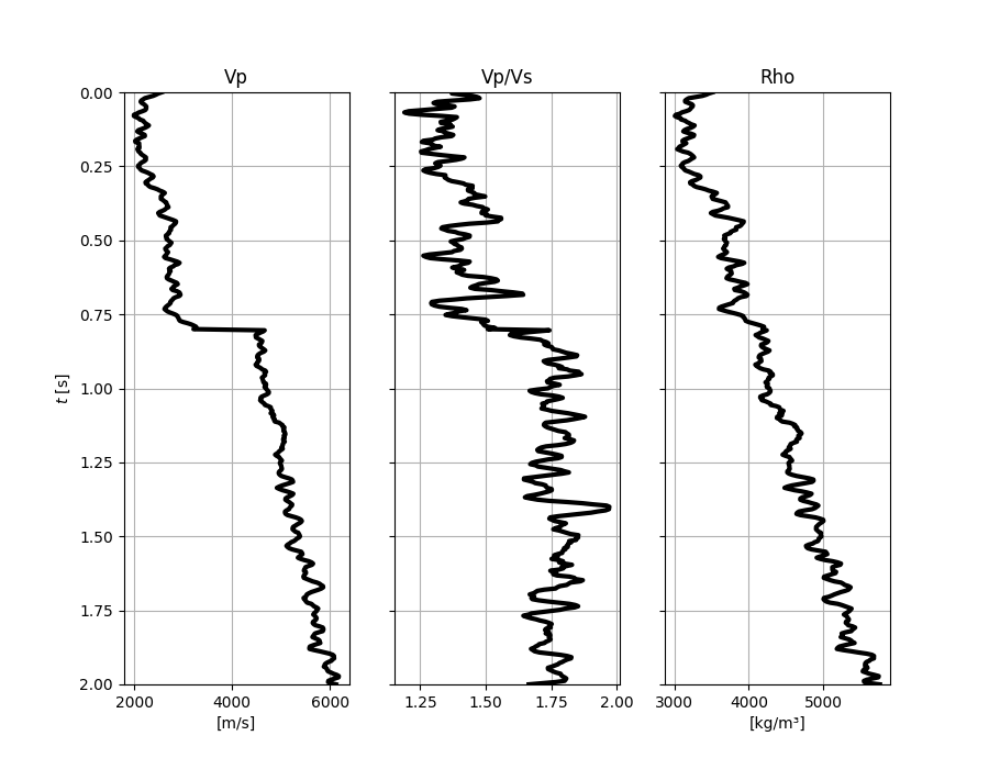
Let’s start by creating the input elastic property profiles

nt0 = 501
dt0 = 0.004
ntheta = 21

t0 = np.arange(nt0) * dt0
thetamin, thetamax = 0.0, 40.0
theta = np.linspace(thetamin, thetamax, ntheta)

# Elastic property profiles
vp = (
    2000
    + 5 * np.arange(nt0)
    + 2 * filtfilt(np.ones(5) / 5.0, 1, np.random.normal(0, 160, nt0))
)
vs = 600 + vp / 2 + 3 * filtfilt(np.ones(5) / 5.0, 1, np.random.normal(0, 100, nt0))
rho = 1000 + vp + filtfilt(np.ones(5) / 5.0, 1, np.random.normal(0, 120, nt0))
vp[201:] += 1500
vs[201:] += 500
rho[201:] += 100

# Wavelet
ntwav = 41
wavoff = 10
wav, twav, wavc = ricker(t0[: ntwav // 2 + 1], 20)
wav_phase = np.hstack((wav[wavoff:], np.zeros(wavoff)))

# vs/vp profile
vsvp = 0.5
vsvp_z = vs / vp

# Model
m = np.stack((np.log(vp), np.log(vs), np.log(rho)), axis=1)

fig, axs = plt.subplots(1, 3, figsize=(9, 7), sharey=True)
axs[0].plot(vp, t0, "k", lw=3)
axs[0].set(xlabel="[m/s]", ylabel=r"$t$ [s]", ylim=[t0[0], t0[-1]], title="Vp")
axs[0].grid()
axs[1].plot(vp / vs, t0, "k", lw=3)
axs[1].set(title="Vp/Vs")
axs[1].grid()
axs[2].plot(rho, t0, "k", lw=3)
axs[2].set(xlabel="[kg/m³]", title="Rho")
axs[2].invert_yaxis()
axs[2].grid()

We create now the operators to model the AVO responses for a set of elastic profiles

# constant vsvp
PPop_const = pylops.avo.avo.AVOLinearModelling(
    theta, vsvp=vsvp, nt0=nt0, linearization="akirich", dtype=np.float64
)

# depth-variant vsvp
PPop_variant = pylops.avo.avo.AVOLinearModelling(
    theta, vsvp=vsvp_z, linearization="akirich", dtype=np.float64
)

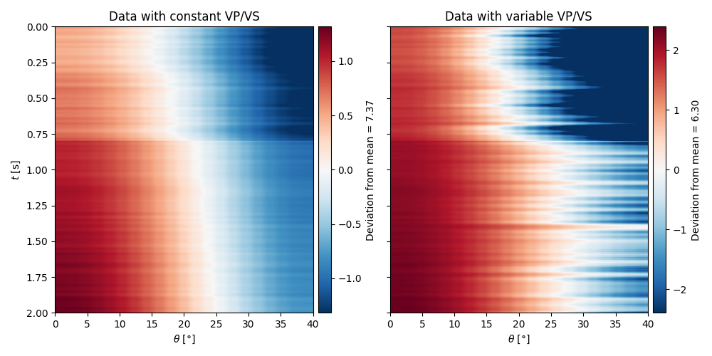
We can then apply those operators to the elastic model and create some synthetic reflection responses

dPP_const = PPop_const * m
dPP_variant = PPop_variant * m

To visualize these responses, we will plot their anomaly - how much they deveiate from their mean

mean_dPP_const = dPP_const.mean()
dPP_const -= mean_dPP_const
mean_dPP_variant = dPP_variant.mean()
dPP_variant -= mean_dPP_variant

fig, axs = plt.subplots(1, 2, figsize=(10, 5), sharey=True)
im = axs[0].imshow(
    dPP_const,
    cmap="RdBu_r",
    extent=(theta[0], theta[-1], t0[-1], t0[0]),
    vmin=-dPP_const.max(),
    vmax=dPP_const.max(),
)
cax = make_axes_locatable(axs[0]).append_axes("right", size="5%", pad="2%")
cb = fig.colorbar(im, cax=cax)
cb.set_label(f"Deviation from mean = {mean_dPP_const:.2f}")
axs[0].set(xlabel=r"$\theta$ [°]", ylabel=r"$t$ [s]", title="Data with constant VP/VS")
axs[0].axis("tight")

im = axs[1].imshow(
    dPP_variant,
    cmap="RdBu_r",
    extent=(theta[0], theta[-1], t0[-1], t0[0]),
    vmin=-dPP_variant.max(),
    vmax=dPP_variant.max(),
)
cax = make_axes_locatable(axs[1]).append_axes("right", size="5%", pad="2%")
cb = fig.colorbar(im, cax=cax)
cb.set_label(f"Deviation from mean = {mean_dPP_variant:.2f}")
axs[1].set(xlabel=r"$\theta$ [°]", title="Data with variable VP/VS")
axs[1].axis("tight")
plt.tight_layout()

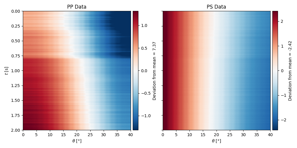
Finally we can also model the PS response by simply changing the linearization choice as follows

PSop = pylops.avo.avo.AVOLinearModelling(
    theta, vsvp=vsvp, nt0=nt0, linearization="ps", dtype=np.float64
)

We can then apply those operators to the elastic model and create some synthetic reflection responses

dPS = PSop * m
mean_dPS = dPS.mean()
dPS -= mean_dPS

fig, axs = plt.subplots(1, 2, figsize=(10, 5), sharey=True)
im = axs[0].imshow(
    dPP_const,
    cmap="RdBu_r",
    extent=(theta[0], theta[-1], t0[-1], t0[0]),
    vmin=-dPP_const.max(),
    vmax=dPP_const.max(),
)
cax = make_axes_locatable(axs[0]).append_axes("right", size="5%", pad="2%")
cb = fig.colorbar(im, cax=cax)
cb.set_label(f"Deviation from mean = {mean_dPP_const:.2f}")
axs[0].set(xlabel=r"$\theta$ [°]", ylabel=r"$t$ [s]", title="PP Data")
axs[0].axis("tight")

im = axs[1].imshow(
    dPS,
    cmap="RdBu_r",
    extent=(theta[0], theta[-1], t0[-1], t0[0]),
    vmin=-dPS.max(),
    vmax=dPS.max(),
)
cax = make_axes_locatable(axs[1]).append_axes("right", size="5%", pad="2%")
cb = fig.colorbar(im, cax=cax)
cb.set_label(f"Deviation from mean = {mean_dPS:.2f}")
axs[1].set(xlabel=r"$\theta$ [°]", title="PS Data")
axs[1].axis("tight")
plt.tight_layout()