CGLS and LSQR Solvers

This example shows how to use the pylops.optimization.leastsquares.cgls and pylops.optimization.leastsquares.lsqr PyLops solvers to minimize the following cost function:

\[J = \| \mathbf{y} - \mathbf{Ax} \|_2^2 + \epsilon \| \mathbf{x} \|_2^2\]

Note that the LSQR solver behaves in the same way as the scipy’s scipy.sparse.linalg.lsqr solver. However, our solver is also able to operate on cupy arrays and perform computations on a GPU.

import warnings

import matplotlib.pyplot as plt
import numpy as np

import pylops

plt.close("all")
warnings.filterwarnings("ignore")

Let’s define a matrix \(\mathbf{A}\) or size (N and M) and fill the matrix with random numbers

N, M = 20, 10
A = np.random.normal(0, 1, (N, M))
Aop = pylops.MatrixMult(A, dtype="float64")

x = np.ones(M)

We can now use the cgls solver to invert this matrix

y = Aop * x
xest, istop, nit, r1norm, r2norm, cost_cgls = pylops.optimization.basic.cgls(
    Aop, y, x0=np.zeros_like(x), niter=10, tol=1e-10, show=True
)

print(f"x= {x}")
print(f"cgls solution xest= {xest}")

CGLS
-----------------------------------------------------------------
The Operator Op has 20 rows and 10 cols
damp = 0.000000e+00     tol = 1.000000e-10      niter = 10
-----------------------------------------------------------------

    Itn          x[0]              r1norm         r2norm
     1        2.8183e-01         4.2058e+00     4.2058e+00
     2        5.9454e-01         2.6036e+00     2.6036e+00
     3        8.7154e-01         1.2171e+00     1.2171e+00
     4        1.0119e+00         5.5478e-01     5.5478e-01
     5        1.0292e+00         2.2891e-01     2.2891e-01
     6        1.0249e+00         1.3605e-01     1.3605e-01
     7        1.0085e+00         9.0791e-02     9.0791e-02
     8        1.0093e+00         6.4846e-02     6.4846e-02
     9        1.0007e+00         5.9283e-03     5.9283e-03
    10        1.0000e+00         2.1688e-12     2.1688e-12

Iterations = 10        Total time (s) = 0.00
-----------------------------------------------------------------

x= [1. 1. 1. 1. 1. 1. 1. 1. 1. 1.]
cgls solution xest= [1. 1. 1. 1. 1. 1. 1. 1. 1. 1.]

And the lsqr solver to invert this matrix

y = Aop * x
(
    xest,
    istop,
    itn,
    r1norm,
    r2norm,
    anorm,
    acond,
    arnorm,
    xnorm,
    var,
    cost_lsqr,
) = pylops.optimization.basic.lsqr(Aop, y, x0=np.zeros_like(x), niter=10, show=True)

print(f"x= {x}")
print(f"lsqr solution xest= {xest}")

LSQR
------------------------------------------------------------------------------------------
The Operator Op has 20 rows and 10 cols
damp = 0.00000000000000e+00     calc_var =      1
atol = 1.00e-08                 conlim = 1.00e+08
btol = 1.00e-08                 niter =       10
------------------------------------------------------------------------------------------
   Itn     x[0]      r1norm     r2norm   Compatible   LS     Norm A   Cond A
     0  0.0000e+00  1.332e+01  1.332e+01   1.0e+00  3.4e-01
     1  2.8183e-01  4.206e+00  4.206e+00   3.2e-01  2.8e-01  4.8e+00  1.0e+00
     2  5.9454e-01  2.604e+00  2.604e+00   2.0e-01  1.7e-01  7.3e+00  2.1e+00
     3  8.7154e-01  1.217e+00  1.217e+00   9.1e-02  8.6e-02  9.2e+00  3.5e+00
     4  1.0119e+00  5.548e-01  5.548e-01   4.2e-02  3.2e-02  1.1e+01  4.8e+00
     5  1.0292e+00  2.289e-01  2.289e-01   1.7e-02  9.9e-03  1.1e+01  6.1e+00
     6  1.0249e+00  1.360e-01  1.360e-01   1.0e-02  5.3e-03  1.2e+01  7.5e+00
     7  1.0085e+00  9.079e-02  9.079e-02   6.8e-03  3.8e-03  1.3e+01  9.0e+00
     8  1.0093e+00  6.485e-02  6.485e-02   4.9e-03  2.1e-03  1.3e+01  1.1e+01
     9  1.0007e+00  5.928e-03  5.928e-03   4.4e-04  2.5e-04  1.4e+01  1.4e+01
    10  1.0000e+00  3.992e-13  3.992e-13   3.0e-14  4.7e-14  1.4e+01  1.5e+01

LSQR finished, Op x - b is small enough, given atol, btol

istop =       1   r1norm = 4.0e-13   anorm = 1.4e+01   arnorm = 2.9e-12
itn   =      10   r2norm = 4.0e-13   acond = 1.5e+01   xnorm  = 3.2e+00
Total time (s) = 0.00
------------------------------------------------------------------------------------------

x= [1. 1. 1. 1. 1. 1. 1. 1. 1. 1.]
lsqr solution xest= [1. 1. 1. 1. 1. 1. 1. 1. 1. 1.]

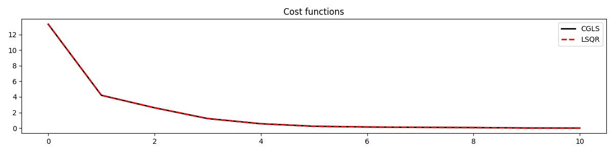
Finally we show that the L2 norm of the residual of the two solvers decays in the same way, as LSQR is algebrically equivalent to CG on the normal equations and CGLS

plt.figure(figsize=(12, 3))
plt.plot(cost_cgls, "k", lw=2, label="CGLS")
plt.plot(cost_lsqr, "--r", lw=2, label="LSQR")
plt.title("Cost functions")
plt.legend()
plt.tight_layout()

Note that while we used a dense matrix here, any other linear operator can be fed to cgls and lsqr as is the case for any other PyLops solver.