Dual-Tree Complex Wavelet Transform

This example shows how to use the pylops.signalprocessing.DTCWT operator to perform the 1D Dual-Tree Complex Wavelet Transform on a (single or multi-dimensional) input array. Such a transform provides advantages over the DWT which lacks shift invariance in 1-D and directional sensitivity in N-D.

import matplotlib.pyplot as plt
import numpy as np
import pywt

import pylops

plt.close("all")

To begin with, let’s define two 1D arrays with a spike at slightly different location

n = 128
x = np.zeros(n)
x1 = np.zeros(n)

x[59] = 1
x1[63] = 1

We now create the DTCWT operator with the shape of our input array. The DTCWT transform provides a Pyramid object that is internally flattened out into a vector. Here we re-obtain the Pyramid object such that we can visualize the different scales indipendently.

level = 3
DCOp = pylops.signalprocessing.DTCWT(dims=n, level=level)
Xc = DCOp.get_pyramid(DCOp @ x)
Xc1 = DCOp.get_pyramid(DCOp @ x1)

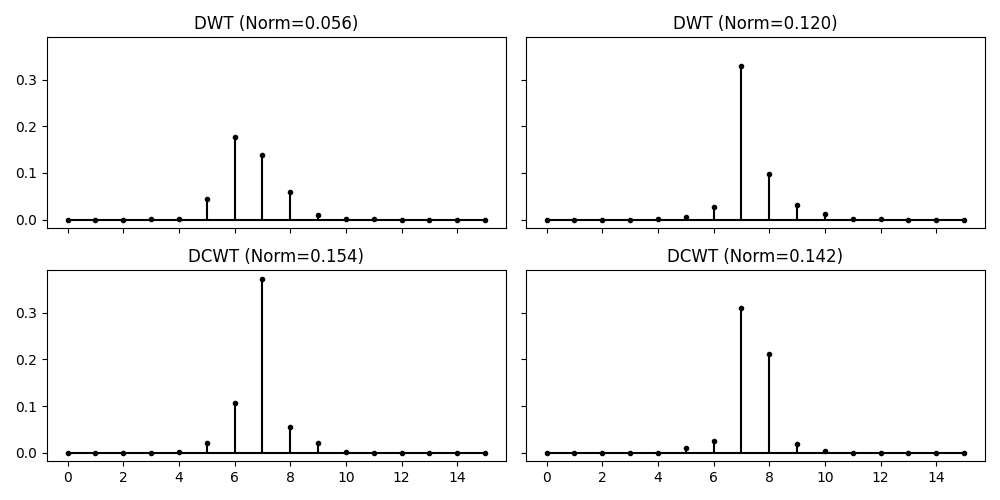
To prove the superiority of the DTCWT transform over the DWT in shift-invariance, let’s also compute the DWT transform of these two signals and compare the coefficents of both transform at level 3. As you will see, the coefficients change completely for the DWT despite the two input signals are very similar; this is not the case for the DCWT transform.

DOp = pylops.signalprocessing.DWT(dims=n, level=level, wavelet="sym7")
X = pywt.array_to_coeffs(DOp @ x, DOp.sl, output_format="wavedecn")
X1 = pywt.array_to_coeffs(DOp @ x1, DOp.sl, output_format="wavedecn")

fig, axs = plt.subplots(2, 2, sharex=True, sharey=True, figsize=(10, 5))
axs[0, 0].stem(np.abs(X[1]["d"]), linefmt="k", markerfmt=".k", basefmt="k")
axs[0, 0].set_title(f"DWT (Norm={np.linalg.norm(np.abs(X[1]['d']))**2:.3f})")
axs[0, 1].stem(np.abs(X1[1]["d"]), linefmt="k", markerfmt=".k", basefmt="k")
axs[0, 1].set_title(f"DWT (Norm={np.linalg.norm(np.abs(X1[1]['d']))**2:.3f})")
axs[1, 0].stem(np.abs(Xc.highpasses[2]), linefmt="k", markerfmt=".k", basefmt="k")
axs[1, 0].set_title(f"DCWT (Norm={np.linalg.norm(np.abs(Xc.highpasses[2]))**2:.3f})")
axs[1, 1].stem(np.abs(Xc1.highpasses[2]), linefmt="k", markerfmt=".k", basefmt="k")
axs[1, 1].set_title(f"DCWT (Norm={np.linalg.norm(np.abs(Xc1.highpasses[2]))**2:.3f})")
plt.tight_layout()

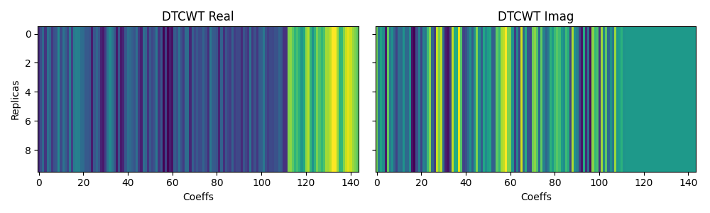
The DTCWT can also be performed on multi-dimension arrays, where the parameter axis is used to define the axis over which the transform is performed. Let’s just replicate our input signal over the second axis and see how the transform will produce the same series of coefficients for all replicas.

nrepeat = 10
x = np.repeat(np.random.rand(n, 1), 10, axis=1).T

level = 3
DCOp = pylops.signalprocessing.DTCWT(dims=(nrepeat, n), level=level, axis=1)
X = DCOp @ x

fig, axs = plt.subplots(1, 2, sharey=True, figsize=(10, 3))
axs[0].imshow(X[0])
axs[0].axis("tight")
axs[0].set_xlabel("Coeffs")
axs[0].set_ylabel("Replicas")
axs[0].set_title("DTCWT Real")
axs[1].imshow(X[1])
axs[1].axis("tight")
axs[1].set_xlabel("Coeffs")
axs[1].set_title("DTCWT Imag")
plt.tight_layout()