Note
Go to the end to download the full example code.
Blending
This example shows how to use the pylops.waveeqprocessing.BlendingContinuous,
pylops.waveeqprocessing.BlendingGroup and
pylops.waveeqprocessing.BlendingHalf operators to blend seismic data
to mimic state-of-the-art simultaneous shooting acquisition systems.
import matplotlib.pyplot as plt
import numpy as np
import scipy as sp

import pylops

plt.close("all")
np.random.seed(0)
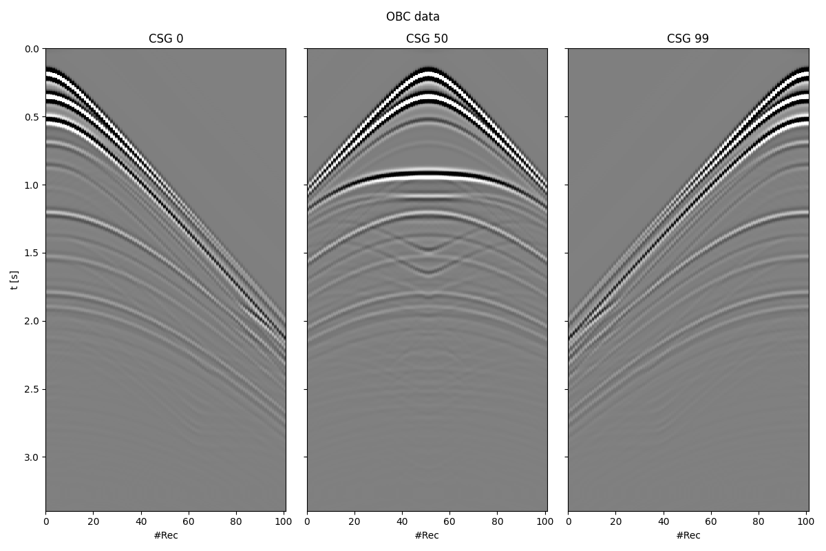
Let’s start by considering a streamer seismic dataset and apply blending in so-called continuous blending mode
inputdata = np.load("../testdata/marchenko/input.npz")
data = inputdata["R"]
data = np.pad(data, ((0, 0), (0, 0), (0, 50)))
wav = inputdata["wav"]
wav_c = np.argmax(wav)
ns, nr, nt = data.shape
# time axis
dt = 0.004
t = np.arange(nt) * dt
# convolve with wavelet
data = np.apply_along_axis(sp.signal.convolve, -1, data, wav, mode="full")
data = data[..., wav_c:][..., :nt]
# obc data
data_obc = data[:-1, :-1]
ns_obc, nr_obc, _ = data_obc.shape
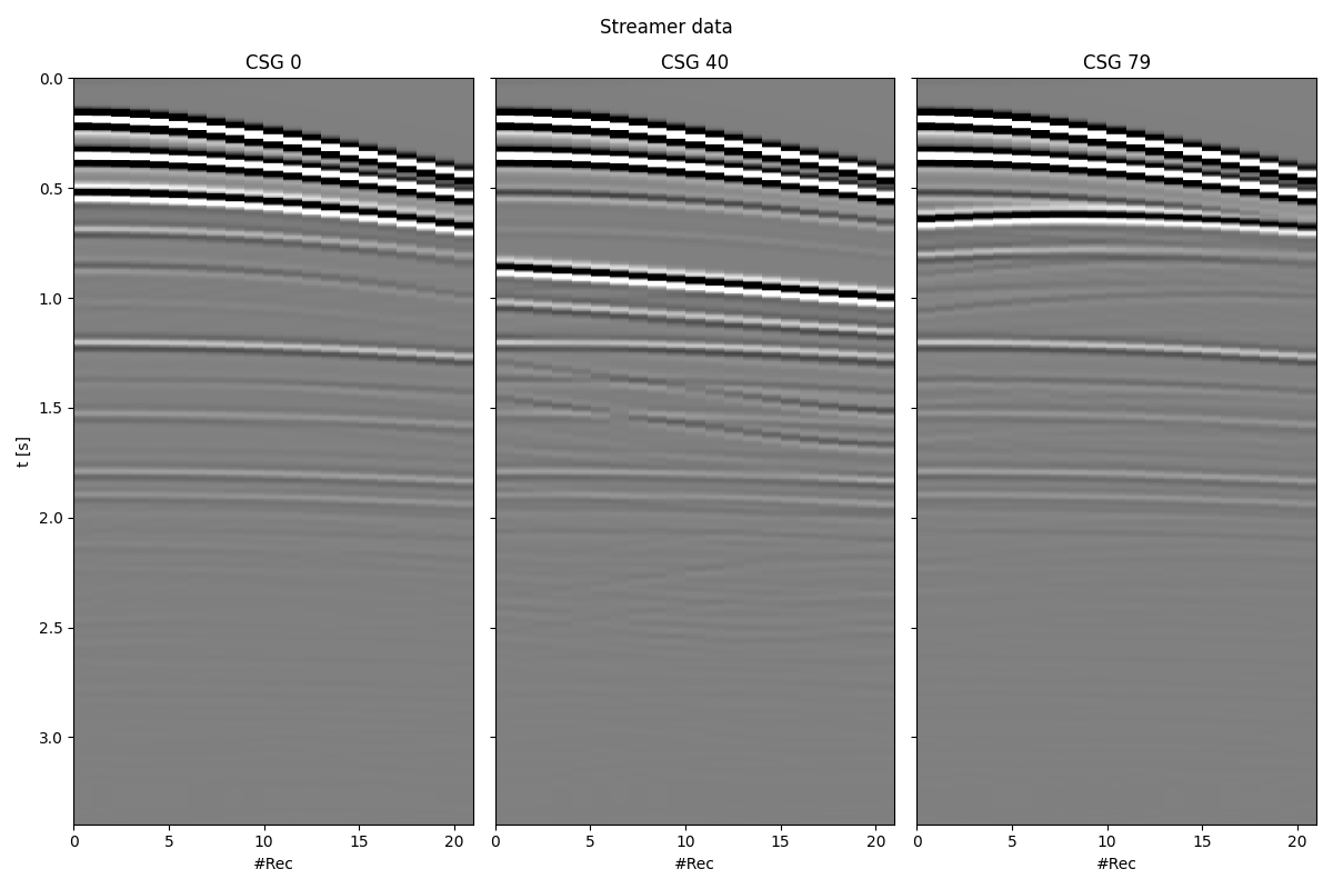
# streamer data
nr_streamer = 21
ns_streamer = ns - nr_streamer
data_streamer = np.zeros((ns_streamer, nr_streamer, nt))
for isrc in range(ns_streamer):
data_streamer[isrc] = data[isrc, isrc : isrc + nr_streamer]
# visualize
isrcplot = [0, ns_obc // 2, ns_obc - 1]
fig, axs = plt.subplots(1, 3, sharey=True, figsize=(12, 8))
fig.suptitle("OBC data")
for i, ax in enumerate(axs):
ax.imshow(
data_obc[isrcplot[i]].T,
cmap="gray",
vmin=-0.1,
vmax=0.1,
extent=(0, nr, t[-1], 0),
interpolation="none",
)
ax.set_title(f"CSG {isrcplot[i]}")
ax.set_xlabel("#Rec")
ax.axis("tight")
axs[0].set_ylabel("t [s]")
plt.tight_layout()
isrcplot = [0, ns_streamer // 2, ns_streamer - 1]
fig, axs = plt.subplots(1, 3, sharey=True, figsize=(12, 8))
fig.suptitle("Streamer data")
for i, ax in enumerate(axs):
ax.imshow(
data_streamer[isrcplot[i]].T,
cmap="gray",
vmin=-0.1,
vmax=0.1,
extent=(0, nr_streamer, t[-1], 0),
interpolation="none",
)
ax.set_title(f"CSG {isrcplot[i]}")
ax.set_xlabel("#Rec")
ax.axis("tight")
axs[0].set_ylabel("t [s]")
plt.tight_layout()
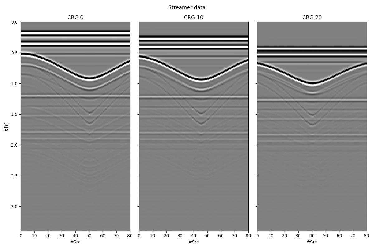
irecplot = [0, nr_streamer // 2, nr_streamer - 1]
fig, axs = plt.subplots(1, 3, sharey=True, figsize=(12, 8))
fig.suptitle("Streamer data")
for i, ax in enumerate(axs):
ax.imshow(
data_streamer[:, irecplot[i]].T,
cmap="gray",
vmin=-0.1,
vmax=0.1,
extent=(0, ns_streamer, t[-1], 0),
interpolation="none",
)
ax.set_title(f"CRG {irecplot[i]}")
ax.set_xlabel("#Src")
ax.axis("tight")
axs[0].set_ylabel("t [s]")
plt.tight_layout()
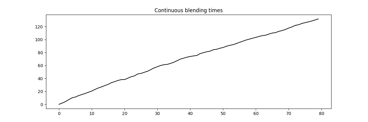
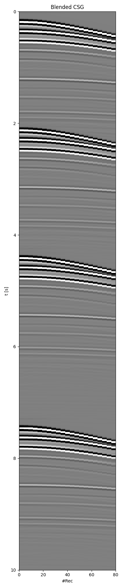
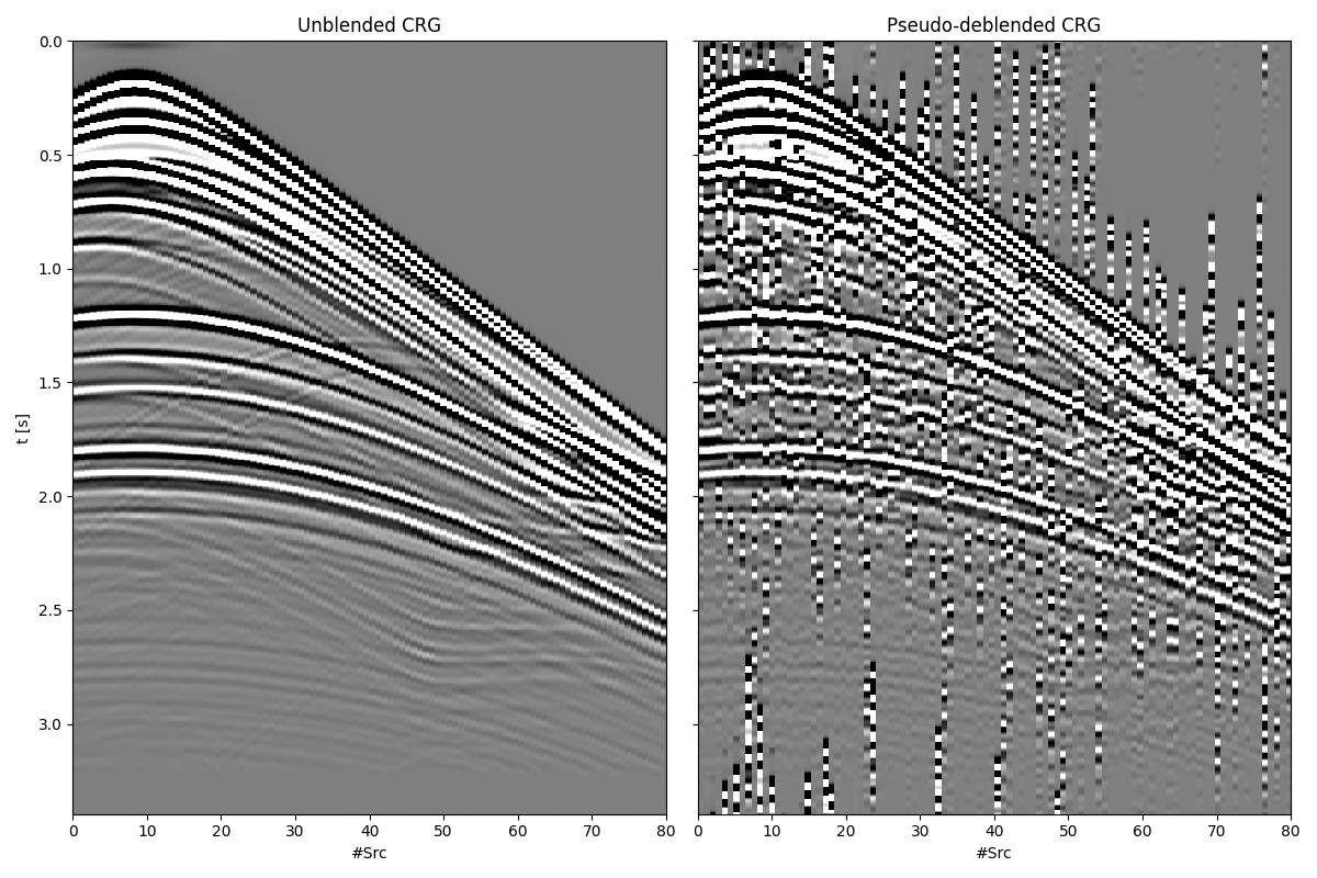
We can now consider the streamer seismic dataset and apply blending in so-called continuous blending mode
overlap = 0.5
ignition_times = np.random.normal(0, 0.6, ns_streamer)
ignition_times += (1 - overlap) * nt * dt
ignition_times[0] = 0.0
ignition_times = np.cumsum(ignition_times)
plt.figure(figsize=(12, 4))
plt.plot(ignition_times, "k")
plt.title("Continuous blending times")
Bop = pylops.waveeqprocessing.BlendingContinuous(
nt,
nr_streamer,
ns_streamer,
dt,
ignition_times,
dtype="complex128",
)
data_blended = Bop * data_streamer
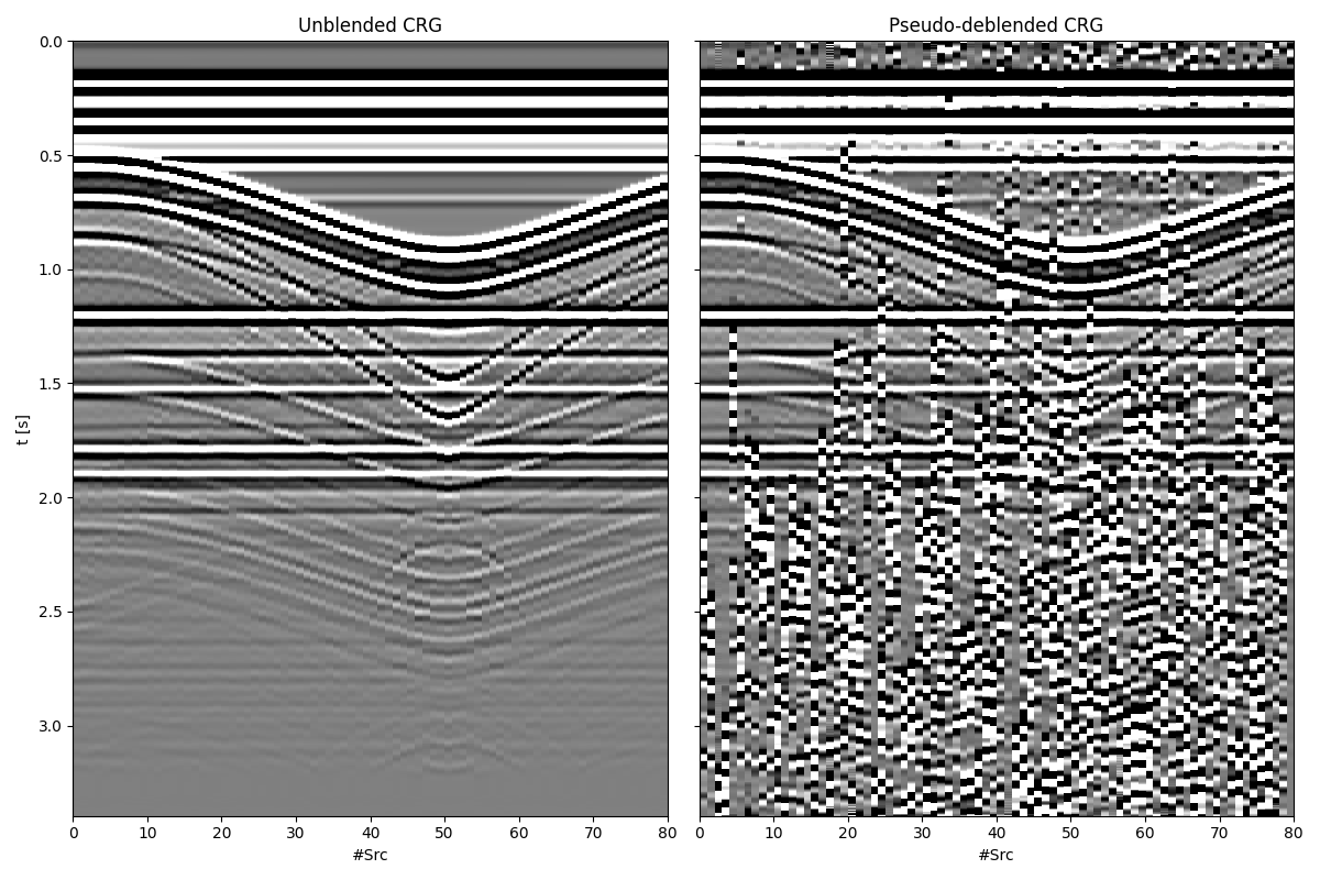
data_pseudo = Bop.H * data_blended
fig, ax = plt.subplots(1, 1, figsize=(4, 19))
ax.imshow(
data_blended.real.T,
cmap="gray",
vmin=-0.1,
vmax=0.1,
extent=(0, ns_streamer, Bop.nttot * dt, 0),
interpolation="none",
)
ax.set_title("Blended CSG")
ax.set_xlabel("#Rec")
ax.set_ylabel("t [s]")
ax.axis("tight")
ax.set_ylim(10, 0)
plt.tight_layout()
fig, axs = plt.subplots(1, 2, sharey=True, figsize=(12, 8))
axs[0].imshow(
data_streamer[:, 0].real.T,
cmap="gray",
vmin=-0.01,
vmax=0.01,
extent=(0, ns_streamer, t[-1], 0),
interpolation="none",
)
axs[0].set_title("Unblended CRG")
axs[0].set_xlabel("#Src")
axs[0].set_ylabel("t [s]")
axs[0].axis("tight")
axs[1].imshow(
data_pseudo[:, 0].real.T,
cmap="gray",
vmin=-0.01,
vmax=0.01,
extent=(0, ns_streamer, t[-1], 0),
interpolation="none",
)
axs[1].set_title("Pseudo-deblended CRG")
axs[1].set_xlabel("#Src")
axs[1].axis("tight")
plt.tight_layout()
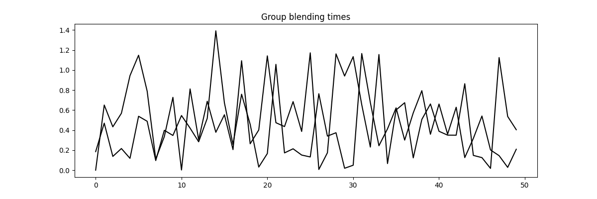
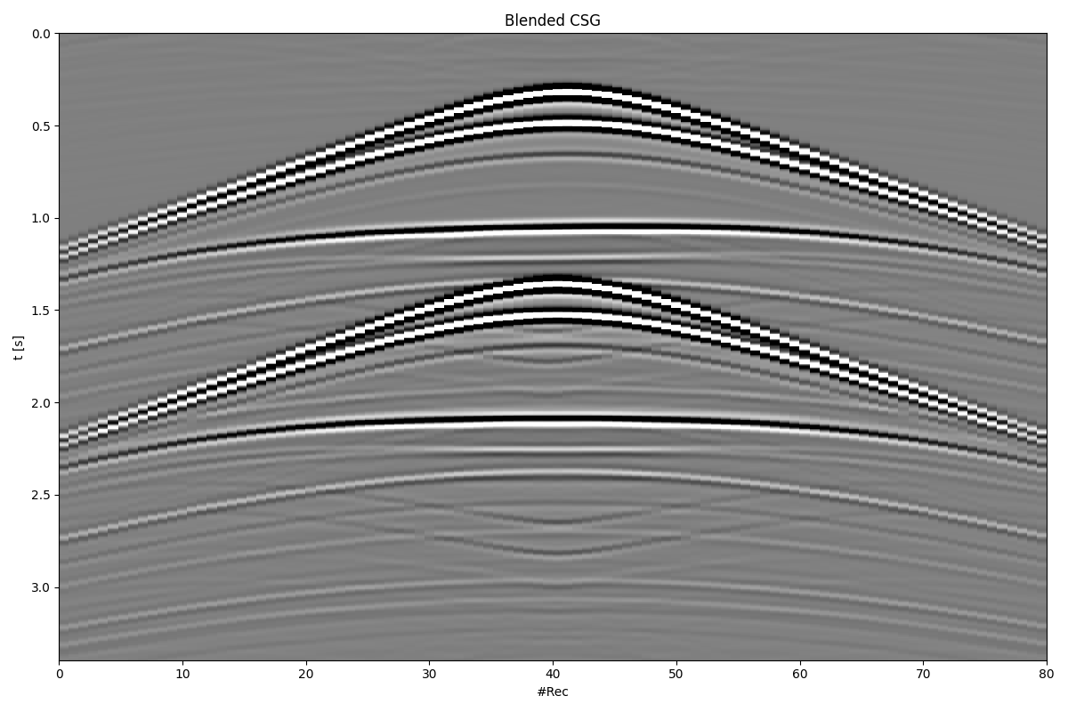
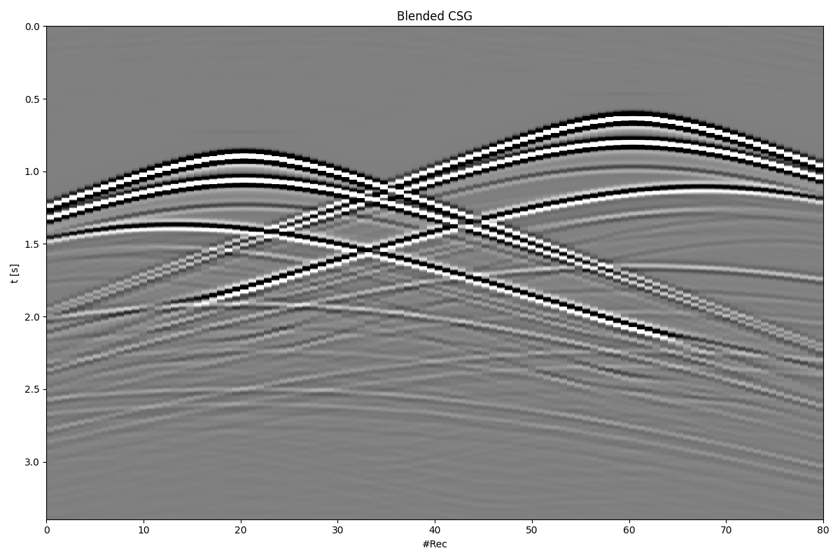
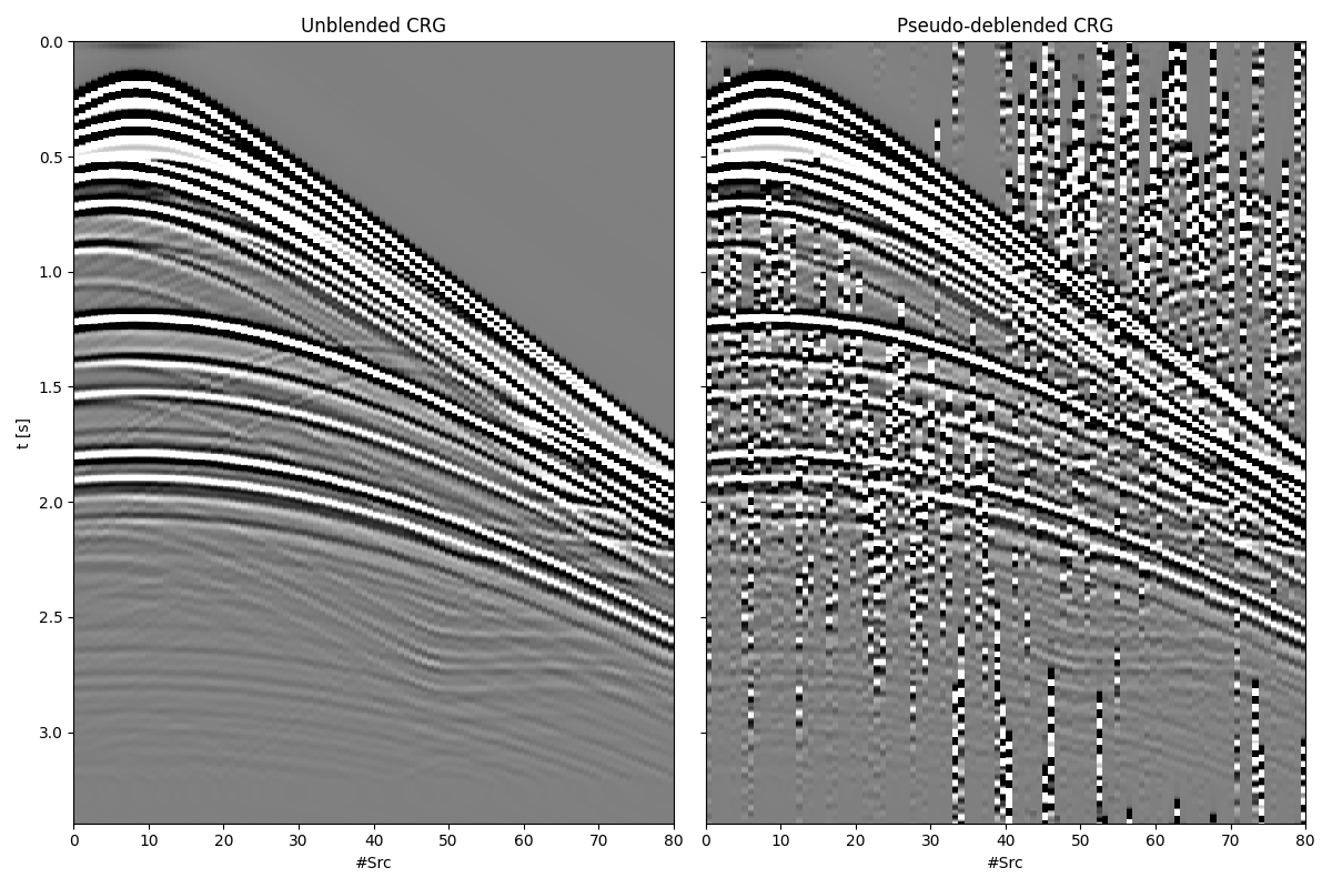
Similarly we can consider the OBC data and apply both group and half blending
# Group
group_size = 2
n_groups = ns_obc // 2
ignition_times = np.abs(np.random.normal(0.2, 0.5, ns_obc)) # only positive shifts
ignition_times[0] = 0.0
plt.figure(figsize=(12, 4))
plt.plot(ignition_times.reshape(group_size, n_groups).T, "k")
plt.title("Group blending times")
Bop = pylops.waveeqprocessing.BlendingGroup(
nt,
nr_obc,
ns_obc,
dt,
ignition_times.reshape(group_size, n_groups),
group_size=group_size,
n_groups=n_groups,
dtype="complex128",
)
data_blended = Bop * data_obc
data_pseudo = Bop.H * data_blended
fig, ax = plt.subplots(1, 1, figsize=(12, 8))
ax.imshow(
data_blended[n_groups // 2].real.T,
cmap="gray",
vmin=-0.1,
vmax=0.1,
extent=(0, ns_streamer, t[-1], 0),
interpolation="none",
)
ax.set_title("Blended CSG")
ax.set_xlabel("#Rec")
ax.set_ylabel("t [s]")
ax.axis("tight")
plt.tight_layout()
fig, axs = plt.subplots(1, 2, sharey=True, figsize=(12, 8))
axs[0].imshow(
data_obc[:, 10].real.T,
cmap="gray",
vmin=-0.01,
vmax=0.01,
extent=(0, ns_streamer, t[-1], 0),
interpolation="none",
)
axs[0].set_title("Unblended CRG")
axs[0].set_xlabel("#Src")
axs[0].set_ylabel("t [s]")
axs[0].axis("tight")
axs[1].imshow(
data_pseudo[:, 10].real.T,
cmap="gray",
vmin=-0.01,
vmax=0.01,
extent=(0, ns_streamer, t[-1], 0),
interpolation="none",
)
axs[1].set_title("Pseudo-deblended CRG")
axs[1].set_xlabel("#Src")
axs[1].axis("tight")
plt.tight_layout()
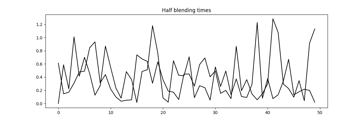
# Half
group_size = 2
n_groups = ns_obc // 2
ignition_times = np.abs(np.random.normal(0.1, 0.5, ns_obc)) # only positive shifts
ignition_times[0] = 0.0
plt.figure(figsize=(12, 4))
plt.plot(ignition_times.reshape(group_size, n_groups).T, "k")
plt.title("Half blending times")
Bop = pylops.waveeqprocessing.BlendingHalf(
nt,
nr_obc,
ns_obc,
dt,
ignition_times.reshape(group_size, n_groups),
group_size=group_size,
n_groups=n_groups,
dtype="complex128",
name=None,
)
data_blended = Bop * data_obc
data_pseudo = Bop.H * data_blended
fig, ax = plt.subplots(1, 1, figsize=(12, 8))
ax.imshow(
data_blended[n_groups // 2].real.T,
cmap="gray",
vmin=-0.1,
vmax=0.1,
extent=(0, ns_streamer, t[-1], 0),
interpolation="none",
)
ax.set_title("Blended CSG")
ax.set_xlabel("#Rec")
ax.set_ylabel("t [s]")
ax.axis("tight")
plt.tight_layout()
fig, axs = plt.subplots(1, 2, sharey=True, figsize=(12, 8))
axs[0].imshow(
data_obc[:, 10].real.T,
cmap="gray",
vmin=-0.01,
vmax=0.01,
extent=(0, ns_streamer, t[-1], 0),
interpolation="none",
)
axs[0].set_title("Unblended CRG")
axs[0].set_xlabel("#Src")
axs[0].set_ylabel("t [s]")
axs[0].axis("tight")
axs[1].imshow(
data_pseudo[:, 10].real.T,
cmap="gray",
vmin=-0.01,
vmax=0.01,
extent=(0, ns_streamer, t[-1], 0),
interpolation="none",
)
axs[1].set_title("Pseudo-deblended CRG")
axs[1].set_xlabel("#Src")
axs[1].axis("tight")
plt.tight_layout()
Total running time of the script: (0 minutes 4.490 seconds)