06. 2D Interpolation

In the mathematical field of numerical analysis, interpolation is the problem of constructing new data points within the range of a discrete set of known data points. In signal and image processing, the data may be recorded at irregular locations and it is often required to regularize the data into a regular grid.

In this tutorial, an example of 2d interpolation of an image is carried out using a combination of PyLops operators (pylops.Restriction and pylops.Laplacian) and the pylops.optimization module.

Mathematically speaking, if we want to interpolate a signal using the theory of inverse problems, we can define the following forward problem:

\[\mathbf{y} = \mathbf{R} \mathbf{x}\]

where the restriction operator \(\mathbf{R}\) selects \(M\) elements from the regularly sampled signal \(\mathbf{x}\) at random locations. The input and output signals are:

\[\mathbf{y}= [y_1, y_2,\ldots,y_N]^T, \qquad \mathbf{x}= [x_1, x_2,\ldots,x_M]^T, \qquad\]

with \(M \gg N\).

import matplotlib.pyplot as plt
import numpy as np

import pylops

plt.close("all")
np.random.seed(0)

To start we import a 2d image and define our restriction operator to irregularly and randomly sample the image for 30% of the entire grid

im = np.load("../testdata/python.npy")[:, :, 0]

Nz, Nx = im.shape
N = Nz * Nx

# Subsample signal
perc_subsampling = 0.2

Nsub2d = int(np.round(N * perc_subsampling))
iava = np.sort(np.random.permutation(np.arange(N))[:Nsub2d])

# Create operators and data
Rop = pylops.Restriction(N, iava, dtype="float64")
D2op = pylops.Laplacian((Nz, Nx), weights=(1, 1), dtype="float64")

x = im.ravel()
y = Rop * x
y1 = Rop.mask(x)

We will now use two different routines from our optimization toolbox to estimate our original image in the regular grid.

xcg_reg_lop = pylops.optimization.leastsquares.normal_equations_inversion(
    Rop, y, [D2op], epsRs=[np.sqrt(0.1)], **dict(maxiter=200)
)[0]

# Invert for interpolated signal, lsqrt
xlsqr_reg_lop = pylops.optimization.leastsquares.regularized_inversion(
    Rop,
    y,
    [D2op],
    epsRs=[np.sqrt(0.1)],
    **dict(damp=0, iter_lim=200, show=0),
)[0]

# Reshape estimated images
im_sampled = y1.reshape((Nz, Nx))
im_rec_lap_cg = xcg_reg_lop.reshape((Nz, Nx))
im_rec_lap_lsqr = xlsqr_reg_lop.reshape((Nz, Nx))

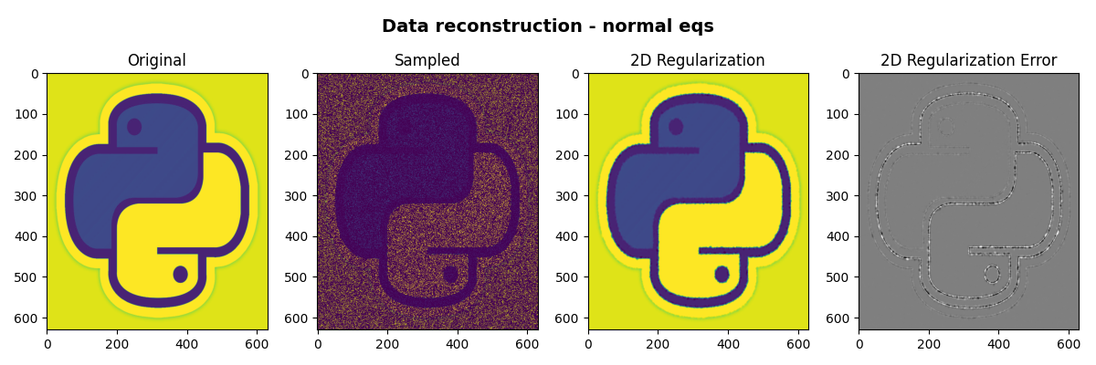
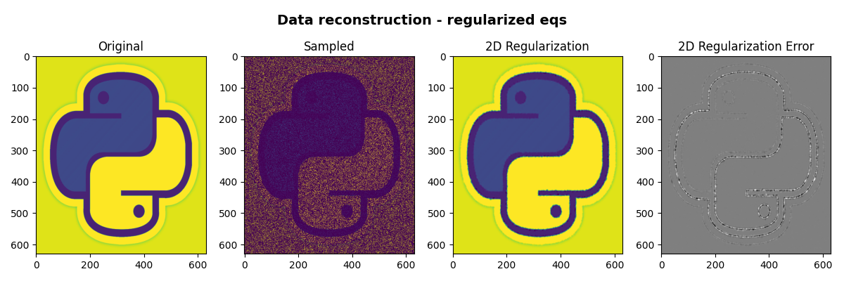
Finally we visualize the original image, the reconstructed images and their error

fig, axs = plt.subplots(1, 4, figsize=(12, 4))
fig.suptitle("Data reconstruction - normal eqs", fontsize=14, fontweight="bold", y=0.95)
axs[0].imshow(im, cmap="viridis", vmin=0, vmax=250)
axs[0].axis("tight")
axs[0].set_title("Original")
axs[1].imshow(im_sampled.data, cmap="viridis", vmin=0, vmax=250)
axs[1].axis("tight")
axs[1].set_title("Sampled")
axs[2].imshow(im_rec_lap_cg, cmap="viridis", vmin=0, vmax=250)
axs[2].axis("tight")
axs[2].set_title("2D Regularization")
axs[3].imshow(im - im_rec_lap_cg, cmap="gray", vmin=-80, vmax=80)
axs[3].axis("tight")
axs[3].set_title("2D Regularization Error")
plt.tight_layout()
plt.subplots_adjust(top=0.8)

fig, axs = plt.subplots(1, 4, figsize=(12, 4))
fig.suptitle(
    "Data reconstruction - regularized eqs", fontsize=14, fontweight="bold", y=0.95
)
axs[0].imshow(im, cmap="viridis", vmin=0, vmax=250)
axs[0].axis("tight")
axs[0].set_title("Original")
axs[1].imshow(im_sampled.data, cmap="viridis", vmin=0, vmax=250)
axs[1].axis("tight")
axs[1].set_title("Sampled")
axs[2].imshow(im_rec_lap_lsqr, cmap="viridis", vmin=0, vmax=250)
axs[2].axis("tight")
axs[2].set_title("2D Regularization")
axs[3].imshow(im - im_rec_lap_lsqr, cmap="gray", vmin=-80, vmax=80)
axs[3].axis("tight")
axs[3].set_title("2D Regularization Error")
plt.tight_layout()
plt.subplots_adjust(top=0.8)

• 
•