Non-stationary Filter Estimation

This example shows how to use the pylops.signalprocessing.NonStationaryFilters1D and pylops.signalprocessing.NonStationaryFilters2D operators to perform non-stationary filter estimation that when convolved with an input signal produces a desired output signal.

import matplotlib.pyplot as plt
import numpy as np
from scipy.signal.windows import gaussian

import pylops
from pylops.utils.wavelets import ricker

plt.close("all")

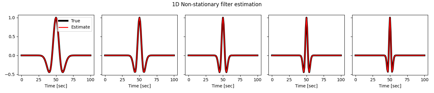
We will start by creating a zero signal of length nt and we will place a comb of unitary spikes. We also create a non-stationary filter defined by 5 equally spaced Ricker wavelets with dominant frequencies of \(f = 10, 15, 20, 25\) and \(30\) Hz.

nt = 601
dt = 0.004
t = np.arange(nt) * dt
tw = ricker(t[:51], f0=5)[1]

fs = [10, 15, 20, 25, 30]
wavs = np.stack([ricker(t[:51], f0=f)[0] for f in fs])

x = np.zeros(nt)
x[64 : nt - 64 : 64] = 1.0

Cop = pylops.signalprocessing.NonStationaryFilters1D(
    x, hsize=101, ih=(101, 201, 301, 401, 501)
)

y = Cop @ wavs

wavsinv = Cop.div(y, niter=20)
wavsinv = wavsinv.reshape(wavs.shape)

fig, axs = plt.subplots(1, len(fs), sharey=True, figsize=(14, 3))
fig.suptitle("1D Non-stationary filter estimation")
for i, ax in enumerate(axs):
    ax.plot(wavs[i], "k", lw=4, label="True")
    ax.plot(wavsinv[i], "r", lw=2, label="Estimate")
    ax.set_xlabel("Time [sec]")
axs[0].legend()
plt.tight_layout()

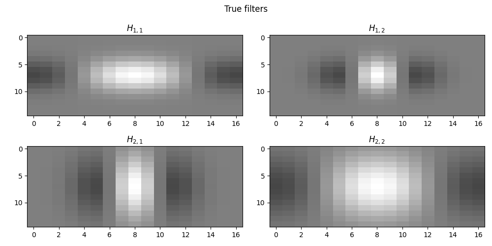
Finally, we repeat the same exercise with a 2-dimensional non-stationary filter

nx, nz = 201, 101

wav1a, _, _ = ricker(t[:9], f0=12)
wav1b, _, _ = ricker(t[:9], f0=30)
wav2a = gaussian(15, 2.0)
wav2b = gaussian(15, 4.0)

wav11 = np.outer(wav1a, wav2a[np.newaxis]).T
wav12 = np.outer(wav1b, wav2a[np.newaxis]).T
wav21 = np.outer(wav1b, wav2b[np.newaxis]).T
wav22 = np.outer(wav1a, wav2b[np.newaxis]).T
wavsize = wav11.shape

hs = np.zeros((2, 2, *wavsize))
hs[0, 0] = wav11
hs[0, 1] = wav12
hs[1, 0] = wav21
hs[1, 1] = wav22

x = np.zeros((nx, nz))
x[:, 21] = 1.0
x[:, 41] = -1.0

Cop = pylops.signalprocessing.NonStationaryFilters2D(
    inp=x, hshape=wavsize, ihx=(21, 41), ihz=(21, 41), engine="numpy"
)

y = Cop @ hs

hsinv = Cop.div(y.ravel(), niter=50)
hsinv = hsinv.reshape(hs.shape)

fig, axs = plt.subplots(2, 2, figsize=(10, 5))
fig.suptitle("True filters")
axs[0, 0].imshow(hs[0, 0], cmap="gray", vmin=-1, vmax=1)
axs[0, 0].axis("tight")
axs[0, 0].set_title(r"$H_{1,1}$")
axs[0, 1].imshow(hs[0, 1], cmap="gray", vmin=-1, vmax=1)
axs[0, 1].axis("tight")
axs[0, 1].set_title(r"$H_{1,2}$")
axs[1, 0].imshow(hs[1, 0], cmap="gray", vmin=-1, vmax=1)
axs[1, 0].axis("tight")
axs[1, 0].set_title(r"$H_{2,1}$")
axs[1, 1].imshow(hs[1, 1], cmap="gray", vmin=-1, vmax=1)
axs[1, 1].axis("tight")
axs[1, 1].set_title(r"$H_{2,2}$")
plt.tight_layout()

fig, axs = plt.subplots(2, 2, figsize=(10, 5))
fig.suptitle("Estimated filters")
axs[0, 0].imshow(hsinv[0, 0], cmap="gray", vmin=-1, vmax=1)
axs[0, 0].axis("tight")
axs[0, 0].set_title(r"$H_{1,1}$")
axs[0, 1].imshow(hsinv[0, 1], cmap="gray", vmin=-1, vmax=1)
axs[0, 1].axis("tight")
axs[0, 1].set_title(r"$H_{1,2}$")
axs[1, 0].imshow(hsinv[1, 0], cmap="gray", vmin=-1, vmax=1)
axs[1, 0].axis("tight")
axs[1, 0].set_title(r"$H_{2,1}$")
axs[1, 1].imshow(hsinv[1, 1], cmap="gray", vmin=-1, vmax=1)
axs[1, 1].axis("tight")
axs[1, 1].set_title(r"$H_{2,2}$")
plt.tight_layout()

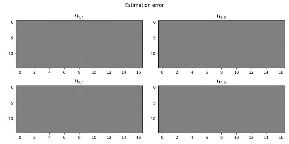
fig, axs = plt.subplots(2, 2, figsize=(10, 5))
fig.suptitle("Estimation error")
axs[0, 0].imshow(hs[0, 0] - hsinv[0, 0], cmap="gray", vmin=-1, vmax=1)
axs[0, 0].axis("tight")
axs[0, 0].set_title(r"$H_{1,1}$")
axs[0, 1].imshow(hs[0, 1] - hsinv[0, 1], cmap="gray", vmin=-1, vmax=1)
axs[0, 1].axis("tight")
axs[0, 1].set_title(r"$H_{1,2}$")
axs[1, 0].imshow(hs[1, 0] - hsinv[1, 0], cmap="gray", vmin=-1, vmax=1)
axs[1, 0].axis("tight")
axs[1, 0].set_title(r"$H_{2,1}$")
axs[1, 1].imshow(hs[1, 1] - hsinv[1, 1], cmap="gray", vmin=-1, vmax=1)
axs[1, 1].axis("tight")
axs[1, 1].set_title(r"$H_{2,2}$")
plt.tight_layout()

• 
• 
•