L1-L1 IRLS

This example shows how to use the pylops.optimization.sparsity.irls solver to solve problems in the form:

\[J = \left\| \mathbf{y}-\mathbf{Ax}\right\|_{1} + \epsilon \left\|\mathbf{x}\right\|_{1}\]

This can be easily achieved by recasting the problem into this equivalent formulation:

\[\begin{split}J = \left\|\left[\begin{array}{c} \mathbf{A} \\ \epsilon \mathbf{I} \end{array}\right] \mathbf{x}-\left[\begin{array}{l} \mathbf{y} \\ \mathbf{0} \end{array}\right]\right\|_{1}\end{split}\]

and solving it using the classical version of the IRLS solver with L1 norm on the data term. In PyLops, the creation of the augmented system happens under the hood when users provide the following optional parameter (kind="datamodel") to the solver.

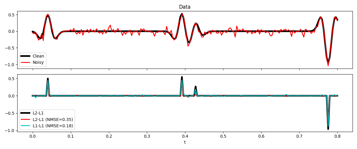
We will now consider a 1D deconvolution problem where the signal is contaminated with Laplace noise. We will compare the classical L2-L1 IRLS solver that works optimally under the condition of Gaussian noise with the above descrived L1-L1 IRLS solver that is best suited to the case of Laplace noise.

import random

import matplotlib.pyplot as plt
import numpy as np

import pylops

plt.close("all")
np.random.seed(10)
random.seed(0)

Let’s start by creating a spiky input signal and convolving it with a Ricker wavelet.

dt = 0.004
nt = 201
t = np.arange(nt) * dt

nspikes = 5
x = np.zeros(nt)
x[random.sample(range(0, nt - 1), nspikes)] = -1 + 2 * np.random.rand(nspikes)

h, th, hcenter = pylops.utils.wavelets.ricker(t[:101], f0=20)
Cop = pylops.signalprocessing.Convolve1D(nt, h=h, offset=hcenter)

y = Cop @ x

We add now a realization of Laplace-distributed noise to our signal and perform a standard spiky deconvolution

yn = y + np.random.laplace(loc=0.0, scale=0.05, size=y.shape)

xl2l1 = pylops.optimization.sparsity.irls(
    Cop,
    yn,
    threshR=True,
    kind="model",
    nouter=100,
    epsR=1e-4,
    epsI=1.0,
    warm=True,
    **dict(iter_lim=100),
)[0]

xl1l1 = pylops.optimization.sparsity.irls(
    Cop,
    yn,
    threshR=True,
    kind="datamodel",
    nouter=100,
    epsR=1e-4,
    epsI=1.0,
    warm=True,
    **dict(iter_lim=100),
)[0]

fig, axs = plt.subplots(2, 1, sharex=True, figsize=(12, 5))
axs[0].plot(t, y, "k", lw=4, label="Clean")
axs[0].plot(t, yn, "r", lw=2, label="Noisy")
axs[0].legend()
axs[0].set_title("Data")
axs[1].plot(t, x, "k", lw=4, label="L2-L1")
axs[1].plot(
    t,
    xl2l1,
    "r",
    lw=2,
    label=f"L2-L1 (NMSE={(np.linalg.norm(xl2l1 - x)/np.linalg.norm(x)):.2f})",
)
axs[1].plot(
    t,
    xl1l1,
    "c",
    lw=2,
    label=f"L1-L1 (NMSE={(np.linalg.norm(xl1l1 - x)/np.linalg.norm(x)):.2f})",
)
axs[1].legend()
axs[1].set_xlabel("t")
plt.tight_layout()