Convolution

This example shows how to use the pylops.signalprocessing.Convolve1D, pylops.signalprocessing.Convolve2D and pylops.signalprocessing.ConvolveND operators to perform convolution between two signals.

Such operators can be used in the forward model of several common application in signal processing that require filtering of an input signal for the instrument response. Similarly, removing the effect of the instrument response from signal is equivalent to solving linear system of equations based on Convolve1D, Convolve2D or ConvolveND operators. This problem is generally referred to as Deconvolution.

A very practical example of deconvolution can be found in the geophysical processing of seismic data where the effect of the source response (i.e., airgun or vibroseis) should be removed from the recorded signal to be able to better interpret the response of the subsurface. Similar examples can be found in telecommunication and speech analysis.

import matplotlib.pyplot as plt
import numpy as np
from scipy.sparse.linalg import lsqr

import pylops
from pylops.utils.wavelets import ricker

plt.close("all")

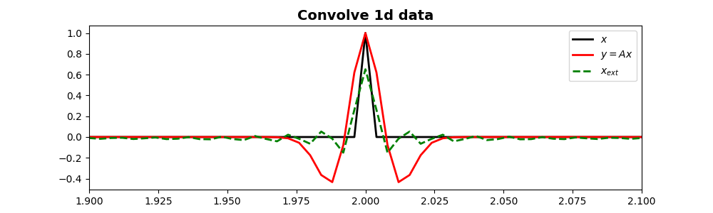
We will start by creating a zero signal of lenght \(nt\) and we will place a unitary spike at its center. We also create our filter to be applied by means of pylops.signalprocessing.Convolve1D operator. Following the seismic example mentioned above, the filter is a Ricker wavelet with dominant frequency \(f_0 = 30 Hz\).

nt = 1001
dt = 0.004
t = np.arange(nt) * dt
x = np.zeros(nt)
x[int(nt / 2)] = 1
h, th, hcenter = ricker(t[:101], f0=30)

Cop = pylops.signalprocessing.Convolve1D(nt, h=h, offset=hcenter, dtype="float32")
y = Cop * x

xinv = Cop / y

fig, ax = plt.subplots(1, 1, figsize=(10, 3))
ax.plot(t, x, "k", lw=2, label=r"$x$")
ax.plot(t, y, "r", lw=2, label=r"$y=Ax$")
ax.plot(t, xinv, "--g", lw=2, label=r"$x_{ext}$")
ax.set_title("Convolve 1d data", fontsize=14, fontweight="bold")
ax.legend()
ax.set_xlim(1.9, 2.1)

Out:

(1.9, 2.1)

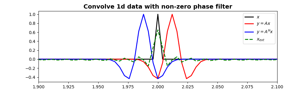
We show now that also a filter with mixed phase (i.e., not centered around zero) can be applied and inverted for using the pylops.signalprocessing.Convolve1D operator.

Cop = pylops.signalprocessing.Convolve1D(nt, h=h, offset=hcenter - 3, dtype="float32")
y = Cop * x
y1 = Cop.H * x
xinv = Cop / y

fig, ax = plt.subplots(1, 1, figsize=(10, 3))
ax.plot(t, x, "k", lw=2, label=r"$x$")
ax.plot(t, y, "r", lw=2, label=r"$y=Ax$")
ax.plot(t, y1, "b", lw=2, label=r"$y=A^Hx$")
ax.plot(t, xinv, "--g", lw=2, label=r"$x_{ext}$")
ax.set_title(
    "Convolve 1d data with non-zero phase filter", fontsize=14, fontweight="bold"
)
ax.set_xlim(1.9, 2.1)
ax.legend()

Out:

<matplotlib.legend.Legend object at 0x7f6af6674cf8>

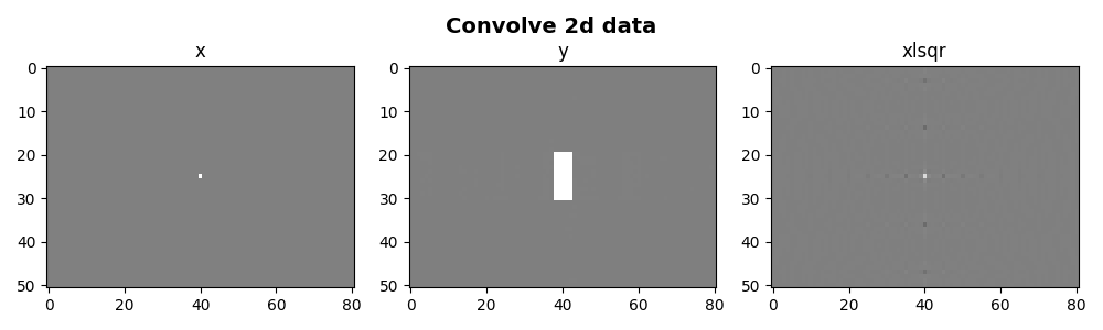
We repeat a similar exercise but using two dimensional signals and filters taking advantage of the pylops.signalprocessing.Convolve2D operator.

nt = 51
nx = 81
dt = 0.004
t = np.arange(nt) * dt
x = np.zeros((nt, nx))
x[int(nt / 2), int(nx / 2)] = 1

nh = [11, 5]
h = np.ones((nh[0], nh[1]))

Cop = pylops.signalprocessing.Convolve2D(
    nt * nx,
    h=h,
    offset=(int(nh[0]) / 2, int(nh[1]) / 2),
    dims=(nt, nx),
    dtype="float32",
)
y = Cop * x.ravel()
xinv = Cop / y

y = y.reshape(nt, nx)
xinv = xinv.reshape(nt, nx)

fig, axs = plt.subplots(1, 3, figsize=(10, 3))
fig.suptitle("Convolve 2d data", fontsize=14, fontweight="bold", y=0.95)
axs[0].imshow(x, cmap="gray", vmin=-1, vmax=1)
axs[1].imshow(y, cmap="gray", vmin=-1, vmax=1)
axs[2].imshow(xinv, cmap="gray", vmin=-1, vmax=1)
axs[0].set_title("x")
axs[0].axis("tight")
axs[1].set_title("y")
axs[1].axis("tight")
axs[2].set_title("xlsqr")
axs[2].axis("tight")
plt.tight_layout()
plt.subplots_adjust(top=0.8)

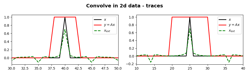
fig, ax = plt.subplots(1, 2, figsize=(10, 3))
fig.suptitle("Convolve in 2d data - traces", fontsize=14, fontweight="bold", y=0.95)
ax[0].plot(x[int(nt / 2), :], "k", lw=2, label=r"$x$")
ax[0].plot(y[int(nt / 2), :], "r", lw=2, label=r"$y=Ax$")
ax[0].plot(xinv[int(nt / 2), :], "--g", lw=2, label=r"$x_{ext}$")
ax[1].plot(x[:, int(nx / 2)], "k", lw=2, label=r"$x$")
ax[1].plot(y[:, int(nx / 2)], "r", lw=2, label=r"$y=Ax$")
ax[1].plot(xinv[:, int(nx / 2)], "--g", lw=2, label=r"$x_{ext}$")
ax[0].legend()
ax[0].set_xlim(30, 50)
ax[1].legend()
ax[1].set_xlim(10, 40)
plt.tight_layout()
plt.subplots_adjust(top=0.8)

• 
• 

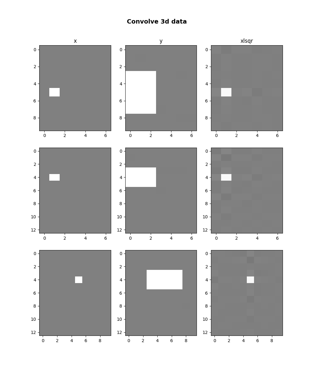
Finally we do the same using three dimensional signals and filters taking advantage of the pylops.signalprocessing.ConvolveND operator.

ny, nx, nz = 13, 10, 7
x = np.zeros((ny, nx, nz))
x[ny // 3, nx // 2, nz // 4] = 1
h = np.ones((3, 5, 3))
offset = [1, 2, 1]

Cop = pylops.signalprocessing.ConvolveND(
    nx * ny * nz, h=h, offset=offset, dims=[ny, nx, nz], dirs=[0, 1, 2], dtype="float32"
)
y = Cop * x.ravel()
xinv = lsqr(Cop, y, damp=0, iter_lim=300, show=0)[0]

y = y.reshape(ny, nx, nz)
xlsqr = xinv.reshape(ny, nx, nz)

fig, axs = plt.subplots(3, 3, figsize=(10, 12))
fig.suptitle("Convolve 3d data", y=0.95, fontsize=14, fontweight="bold")
axs[0][0].imshow(x[ny // 3], cmap="gray", vmin=-1, vmax=1)
axs[0][1].imshow(y[ny // 3], cmap="gray", vmin=-1, vmax=1)
axs[0][2].imshow(xlsqr[ny // 3], cmap="gray", vmin=-1, vmax=1)
axs[0][0].set_title("x")
axs[0][0].axis("tight")
axs[0][1].set_title("y")
axs[0][1].axis("tight")
axs[0][2].set_title("xlsqr")
axs[0][2].axis("tight")
axs[1][0].imshow(x[:, nx // 2], cmap="gray", vmin=-1, vmax=1)
axs[1][1].imshow(y[:, nx // 2], cmap="gray", vmin=-1, vmax=1)
axs[1][2].imshow(xlsqr[:, nx // 2], cmap="gray", vmin=-1, vmax=1)
axs[1][0].axis("tight")
axs[1][1].axis("tight")
axs[1][2].axis("tight")
axs[2][0].imshow(x[..., nz // 4], cmap="gray", vmin=-1, vmax=1)
axs[2][1].imshow(y[..., nz // 4], cmap="gray", vmin=-1, vmax=1)
axs[2][2].imshow(xlsqr[..., nz // 4], cmap="gray", vmin=-1, vmax=1)
axs[2][0].axis("tight")
axs[2][1].axis("tight")
axs[2][2].axis("tight")

Out:

(-0.5, 9.5, 12.5, -0.5)