Radon Transform

This example shows how to use the pylops.signalprocessing.Radon2D and pylops.signalprocessing.Radon3D operators to apply the Radon Transform to 2-dimensional or 3-dimensional signals, respectively. In our implementation both linear, parabolic and hyperbolic parametrization can be chosen.

import matplotlib.pyplot as plt
import numpy as np

import pylops

plt.close("all")

Let’s start by creating an empty 2d matrix of size \(n_{p_x} \times n_t\) and add a single spike in it. We will see that applying the forward Radon operator will result in a single event (linear, parabolic or hyperbolic) in the resulting data vector.

nt, nh = 41, 51
npx, pxmax = 41, 1e-2

dt, dh = 0.005, 1
t = np.arange(nt) * dt
h = np.arange(nh) * dh
px = np.linspace(0, pxmax, npx)

x = np.zeros((npx, nt))
x[4, nt // 2] = 1

We can now define our operators for different parametric curves and apply them to the input model vector. We also apply the adjoint to the resulting data vector.

RLop = pylops.signalprocessing.Radon2D(
    t, h, px, centeredh=True, kind="linear", interp=False, engine="numpy"
)
RPop = pylops.signalprocessing.Radon2D(
    t, h, px, centeredh=True, kind="parabolic", interp=False, engine="numpy"
)
RHop = pylops.signalprocessing.Radon2D(
    t, h, px, centeredh=True, kind="hyperbolic", interp=False, engine="numpy"
)

# forward
yL = RLop * x.ravel()
yP = RPop * x.ravel()
yH = RHop * x.ravel()
yL = yL.reshape(nh, nt)
yP = yP.reshape(nh, nt)
yH = yH.reshape(nh, nt)

# adjoint
xadjL = RLop.H * yL.ravel()
xadjP = RPop.H * yP.ravel()
xadjH = RHop.H * yH.ravel()
xadjL = xadjL.reshape(npx, nt)
xadjP = xadjP.reshape(npx, nt)
xadjH = xadjH.reshape(npx, nt)

Let’s now visualize the input model in the Radon domain, the data, and the adjoint model the different parametric curves.

fig, axs = plt.subplots(2, 4, figsize=(10, 6))
axs[0][0].imshow(
    x.T, vmin=-1, vmax=1, cmap="seismic_r", extent=(px[0], px[-1], t[-1], t[0])
)
axs[0][0].set_title("Input model")
axs[0][0].axis("tight")
axs[0][1].imshow(
    yL.T, vmin=-1, vmax=1, cmap="seismic_r", extent=(h[0], h[-1], t[-1], t[0])
)
axs[0][1].set_title("Linear data")
axs[0][1].axis("tight")
axs[0][2].imshow(
    yP.T, vmin=-1, vmax=1, cmap="seismic_r", extent=(h[0], h[-1], t[-1], t[0])
)
axs[0][2].set_title("Parabolic data")
axs[0][2].axis("tight")
axs[0][3].imshow(
    yH.T, vmin=-1, vmax=1, cmap="seismic_r", extent=(h[0], h[-1], t[-1], t[0])
)
axs[0][3].set_title("Hyperbolic data")
axs[0][3].axis("tight")
axs[1][1].imshow(
    xadjL.T, vmin=-20, vmax=20, cmap="seismic_r", extent=(px[0], px[-1], t[-1], t[0])
)
axs[1][0].axis("off")
axs[1][1].set_title("Linear adjoint")
axs[1][1].axis("tight")
axs[1][2].imshow(
    xadjP.T, vmin=-20, vmax=20, cmap="seismic_r", extent=(px[0], px[-1], t[-1], t[0])
)
axs[1][2].set_title("Parabolic adjoint")
axs[1][2].axis("tight")
axs[1][3].imshow(
    xadjH.T, vmin=-20, vmax=20, cmap="seismic_r", extent=(px[0], px[-1], t[-1], t[0])
)
axs[1][3].set_title("Hyperbolic adjoint")
axs[1][3].axis("tight")
fig.tight_layout()

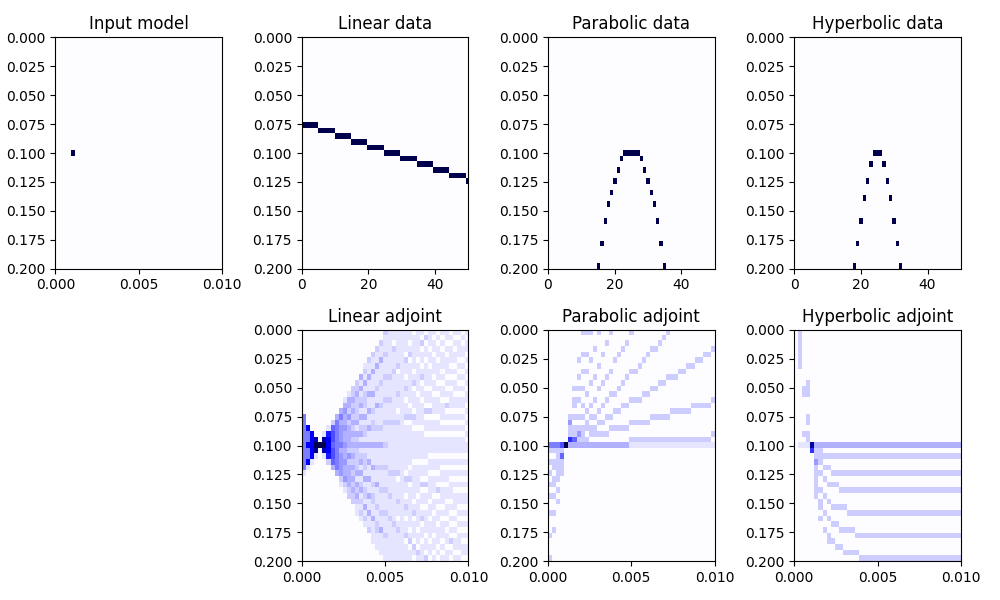
As we can see in the bottom figures, the adjoint Radon transform is far from being close to the inverse Radon transform, i.e. \(\mathbf{R^H}\mathbf{R} \neq \mathbf{I}\) (compared to the case of FFT where the adjoint and inverse are equivalent, i.e. \(\mathbf{F^H}\mathbf{F} = \mathbf{I}\)). In fact when we apply the adjoint Radon Transform we obtain a model that is a smoothed version of the original model polluted by smearing and artifacts. In tutorial 11. Radon filtering we will exploit a sparsity-promiting Radon transform to perform filtering of unwanted signals from an input data.

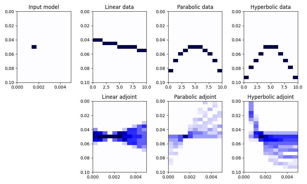
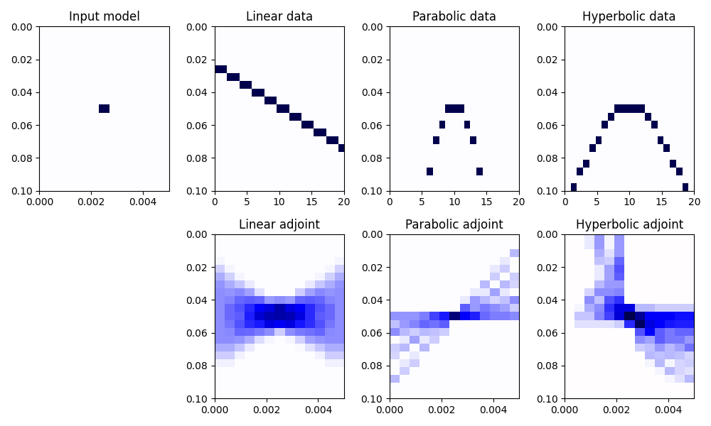
Finally we repeat the same exercise with 3d data.

nt, ny, nx = 21, 21, 11
npy, pymax = 13, 5e-3
npx, pxmax = 11, 5e-3

dt, dy, dx = 0.005, 1, 1
t = np.arange(nt) * dt
hy = np.arange(ny) * dy
hx = np.arange(nx) * dx

py = np.linspace(0, pymax, npy)
px = np.linspace(0, pxmax, npx)

x = np.zeros((npy, npx, nt))
x[npy // 2, npx // 2 - 2, nt // 2] = 1

RLop = pylops.signalprocessing.Radon3D(
    t, hy, hx, py, px, centeredh=True, kind="linear", interp=False, engine="numpy"
)
RPop = pylops.signalprocessing.Radon3D(
    t, hy, hx, py, px, centeredh=True, kind="parabolic", interp=False, engine="numpy"
)
RHop = pylops.signalprocessing.Radon3D(
    t, hy, hx, py, px, centeredh=True, kind="hyperbolic", interp=False, engine="numpy"
)

# forward
yL = RLop * x.ravel()
yP = RPop * x.ravel()
yH = RHop * x.ravel()
yL = yL.reshape(ny, nx, nt)
yP = yP.reshape(ny, nx, nt)
yH = yH.reshape(ny, nx, nt)

# adjoint
xadjL = RLop.H * yL.ravel()
xadjP = RPop.H * yP.ravel()
xadjH = RHop.H * yH.ravel()
xadjL = xadjL.reshape(npy, npx, nt)
xadjP = xadjP.reshape(npy, npx, nt)
xadjH = xadjH.reshape(npy, npx, nt)

# plotting
fig, axs = plt.subplots(2, 4, figsize=(10, 6))
axs[0][0].imshow(
    x[npy // 2].T,
    vmin=-1,
    vmax=1,
    cmap="seismic_r",
    extent=(px[0], px[-1], t[-1], t[0]),
)
axs[0][0].set_title("Input model")
axs[0][0].axis("tight")
axs[0][1].imshow(
    yL[ny // 2].T,
    vmin=-1,
    vmax=1,
    cmap="seismic_r",
    extent=(hx[0], hx[-1], t[-1], t[0]),
)
axs[0][1].set_title("Linear data")
axs[0][1].axis("tight")
axs[0][2].imshow(
    yP[ny // 2].T,
    vmin=-1,
    vmax=1,
    cmap="seismic_r",
    extent=(hx[0], hx[-1], t[-1], t[0]),
)
axs[0][2].set_title("Parabolic data")
axs[0][2].axis("tight")
axs[0][3].imshow(
    yH[ny // 2].T,
    vmin=-1,
    vmax=1,
    cmap="seismic_r",
    extent=(hx[0], hx[-1], t[-1], t[0]),
)
axs[0][3].set_title("Hyperbolic data")
axs[0][3].axis("tight")
axs[1][1].imshow(
    xadjL[npy // 2].T,
    vmin=-100,
    vmax=100,
    cmap="seismic_r",
    extent=(px[0], px[-1], t[-1], t[0]),
)
axs[1][0].axis("off")
axs[1][1].set_title("Linear adjoint")
axs[1][1].axis("tight")
axs[1][2].imshow(
    xadjP[npy // 2].T,
    vmin=-100,
    vmax=100,
    cmap="seismic_r",
    extent=(px[0], px[-1], t[-1], t[0]),
)
axs[1][2].set_title("Parabolic adjoint")
axs[1][2].axis("tight")
axs[1][3].imshow(
    xadjH[npy // 2].T,
    vmin=-100,
    vmax=100,
    cmap="seismic_r",
    extent=(px[0], px[-1], t[-1], t[0]),
)
axs[1][3].set_title("Hyperbolic adjoint")
axs[1][3].axis("tight")
fig.tight_layout()

fig, axs = plt.subplots(2, 4, figsize=(10, 6))
axs[0][0].imshow(
    x[:, npx // 2 - 2].T,
    vmin=-1,
    vmax=1,
    cmap="seismic_r",
    extent=(py[0], py[-1], t[-1], t[0]),
)
axs[0][0].set_title("Input model")
axs[0][0].axis("tight")
axs[0][1].imshow(
    yL[:, nx // 2].T,
    vmin=-1,
    vmax=1,
    cmap="seismic_r",
    extent=(hy[0], hy[-1], t[-1], t[0]),
)
axs[0][1].set_title("Linear data")
axs[0][1].axis("tight")
axs[0][2].imshow(
    yP[:, nx // 2].T,
    vmin=-1,
    vmax=1,
    cmap="seismic_r",
    extent=(hy[0], hy[-1], t[-1], t[0]),
)
axs[0][2].set_title("Parabolic data")
axs[0][2].axis("tight")
axs[0][3].imshow(
    yH[:, nx // 2].T,
    vmin=-1,
    vmax=1,
    cmap="seismic_r",
    extent=(hy[0], hy[-1], t[-1], t[0]),
)
axs[0][3].set_title("Hyperbolic data")
axs[0][3].axis("tight")
axs[1][1].imshow(
    xadjL[:, npx // 2 - 5].T,
    vmin=-100,
    vmax=100,
    cmap="seismic_r",
    extent=(py[0], py[-1], t[-1], t[0]),
)
axs[1][0].axis("off")
axs[1][1].set_title("Linear adjoint")
axs[1][1].axis("tight")
axs[1][2].imshow(
    xadjP[:, npx // 2 - 2].T,
    vmin=-100,
    vmax=100,
    cmap="seismic_r",
    extent=(py[0], py[-1], t[-1], t[0]),
)
axs[1][2].set_title("Parabolic adjoint")
axs[1][2].axis("tight")
axs[1][3].imshow(
    xadjH[:, npx // 2 - 2].T,
    vmin=-100,
    vmax=100,
    cmap="seismic_r",
    extent=(py[0], py[-1], t[-1], t[0]),
)
axs[1][3].set_title("Hyperbolic adjoint")
axs[1][3].axis("tight")
fig.tight_layout()

• 
•