Note
Click here to download the full example code
13. Deghosting
Single-component seismic data can be decomposed
in their up- and down-going constituents in a model driven fashion.
This task can be achieved by defining an f-k propagator (or ghost model) and
solving an inverse problem as described in
pylops.waveeqprocessing.Deghosting.
import matplotlib.pyplot as plt

# sphinx_gallery_thumbnail_number = 3
import numpy as np
from scipy.sparse.linalg import lsqr

import pylops

np.random.seed(0)
plt.close("all")
Let’s start by loading the input dataset and geometry
inputfile = "../testdata/updown/input.npz"
inputdata = np.load(inputfile)
vel_sep = 2400.0 # velocity at separation level
clip = 1e-1 # plotting clip
# Receivers
r = inputdata["r"]
nr = r.shape[1]
dr = r[0, 1] - r[0, 0]
# Sources
s = inputdata["s"]
# Model
rho = inputdata["rho"]
# Axes
t = inputdata["t"]
nt, dt = len(t), t[1] - t[0]
x, z = inputdata["x"], inputdata["z"]
dx, dz = x[1] - x[0], z[1] - z[0]
# Data
p = inputdata["p"].T
p /= p.max()
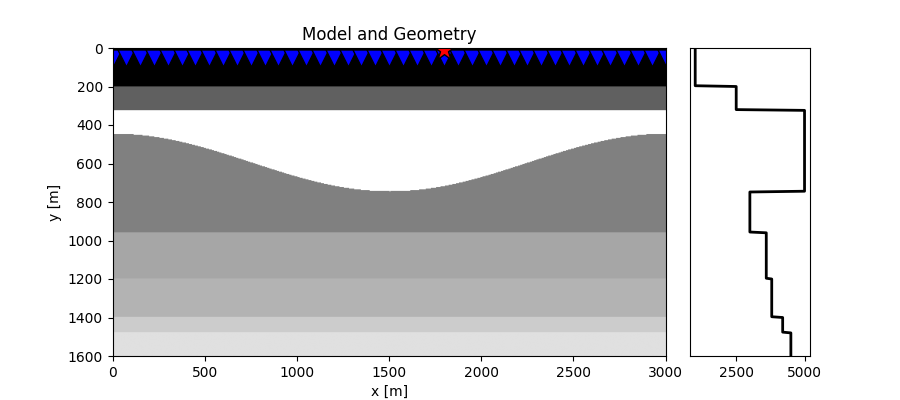
fig = plt.figure(figsize=(9, 4))
ax1 = plt.subplot2grid((1, 5), (0, 0), colspan=4)
ax2 = plt.subplot2grid((1, 5), (0, 4))
ax1.imshow(rho, cmap="gray", extent=(x[0], x[-1], z[-1], z[0]))
ax1.scatter(r[0, ::5], r[1, ::5], marker="v", s=150, c="b", edgecolors="k")
ax1.scatter(s[0], s[1], marker="*", s=250, c="r", edgecolors="k")
ax1.axis("tight")
ax1.set_xlabel("x [m]")
ax1.set_ylabel("y [m]")
ax1.set_title("Model and Geometry")
ax1.set_xlim(x[0], x[-1])
ax1.set_ylim(z[-1], z[0])
ax2.plot(rho[:, len(x) // 2], z, "k", lw=2)
ax2.set_ylim(z[-1], z[0])
ax2.set_yticks([])
Out:
[]
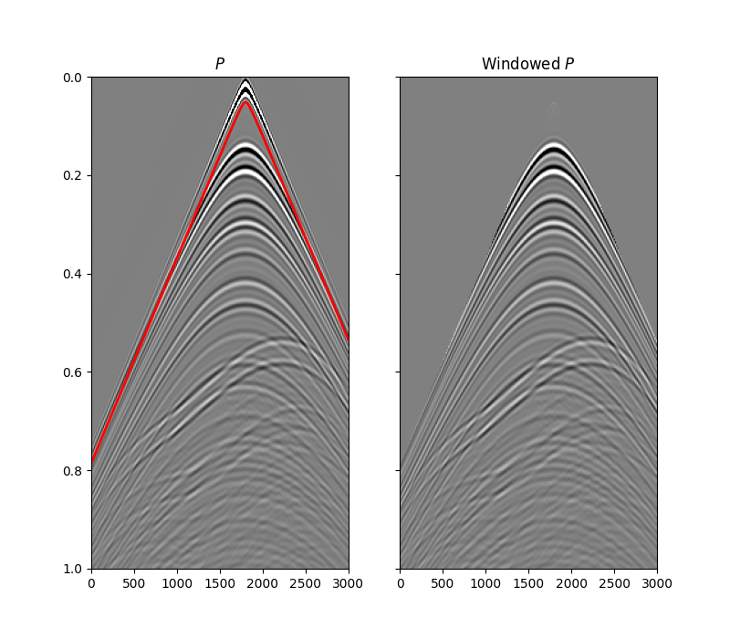
To be able to deghost the input dataset, we need to remove its direct arrival. In this example we will create a mask based on the analytical traveltime of the direct arrival.
direct = np.sqrt(np.sum((s[:, np.newaxis] - r) ** 2, axis=0)) / vel_sep

# Window
off = 0.035
direct_off = direct + off
win = np.zeros((nt, nr))
iwin = np.round(direct_off / dt).astype(int)
for i in range(nr):
    win[iwin[i] :, i] = 1


fig, axs = plt.subplots(1, 2, sharey=True, figsize=(8, 7))
axs[0].imshow(
    p.T,
    cmap="gray",
    vmin=-clip * np.abs(p).max(),
    vmax=clip * np.abs(p).max(),
    extent=(r[0, 0], r[0, -1], t[-1], t[0]),
)
axs[0].plot(r[0], direct_off, "r", lw=2)
axs[0].set_title(r"$P$")
axs[0].axis("tight")
axs[1].imshow(
    win * p.T,
    cmap="gray",
    vmin=-clip * np.abs(p).max(),
    vmax=clip * np.abs(p).max(),
    extent=(r[0, 0], r[0, -1], t[-1], t[0]),
)
axs[1].set_title(r"Windowed $P$")
axs[1].axis("tight")
axs[1].set_ylim(1, 0)
Out:
(1.0, 0.0)
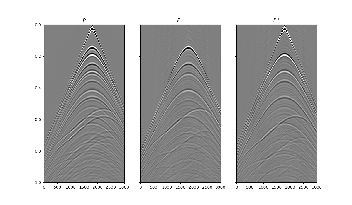
We can now perform deghosting
pup, pdown = pylops.waveeqprocessing.Deghosting(
p.T,
nt,
nr,
dt,
dr,
vel_sep,
r[1, 0] + dz,
win=win,
npad=5,
ntaper=11,
solver=lsqr,
dottest=False,
dtype="complex128",
**dict(damp=1e-10, iter_lim=60)
)
fig, axs = plt.subplots(1, 3, sharey=True, figsize=(12, 7))
axs[0].imshow(
p.T,
cmap="gray",
vmin=-clip * np.abs(p).max(),
vmax=clip * np.abs(p).max(),
extent=(r[0, 0], r[0, -1], t[-1], t[0]),
)
axs[0].set_title(r"$P$")
axs[0].axis("tight")
axs[1].imshow(
pup,
cmap="gray",
vmin=-clip * np.abs(p).max(),
vmax=clip * np.abs(p).max(),
extent=(r[0, 0], r[0, -1], t[-1], t[0]),
)
axs[1].set_title(r"$P^-$")
axs[1].axis("tight")
axs[2].imshow(
pdown,
cmap="gray",
vmin=-clip * np.abs(p).max(),
vmax=clip * np.abs(p).max(),
extent=(r[0, 0], r[0, -1], t[-1], t[0]),
)
axs[2].set_title(r"$P^+$")
axs[2].axis("tight")
axs[2].set_ylim(1, 0)
plt.figure(figsize=(14, 3))
plt.plot(t, p[nr // 2], "k", lw=2, label=r"$p$")
plt.plot(t, pup[:, nr // 2], "r", lw=2, label=r"$p^-$")
plt.xlim(0, t[200])
plt.ylim(-0.2, 0.2)
plt.legend()
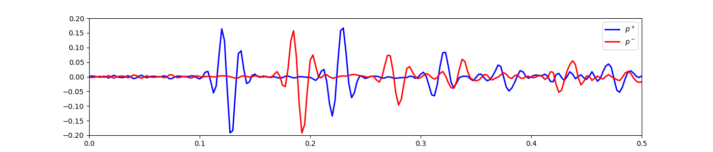
plt.figure(figsize=(14, 3))
plt.plot(t, pdown[:, nr // 2], "b", lw=2, label=r"$p^+$")
plt.plot(t, pup[:, nr // 2], "r", lw=2, label=r"$p^-$")
plt.xlim(0, t[200])
plt.ylim(-0.2, 0.2)
plt.legend()
Out:
<matplotlib.legend.Legend object at 0x7f90cd709400>
To see more examples head over to the following notebook: notebook1.
Total running time of the script: ( 0 minutes 6.727 seconds)