07. Post-stack inversion

Estimating subsurface properties from band-limited seismic data represents an important task for geophysical subsurface characterization.

In this tutorial, the pylops.avo.poststack.PoststackLinearModelling operator is used for modelling of both 1d and 2d synthetic post-stack seismic data from a profile or 2d model of the subsurface acoustic impedence.

\[d(t, \theta=0) = \frac{1}{2} w(t) * \frac{\mathrm{d}\ln \text{AI}(t)}{\mathrm{d}t}\]

where \(\text{AI}(t)\) is the acoustic impedance profile and \(w(t)\) is the time domain seismic wavelet. In compact form:

\[\mathbf{d}= \mathbf{W} \mathbf{D} \mathbf{ai}\]

where \(\mathbf{W}\) is a convolution operator, \(\mathbf{D}\) is a first derivative operator, and \(\mathbf{ai}\) is the input model. Subsequently the acoustic impedance model is estimated via the pylops.avo.poststack.PoststackInversion module. A two-steps inversion strategy is finally presented to deal with the case of noisy data.

import matplotlib.pyplot as plt

# sphinx_gallery_thumbnail_number = 4
import numpy as np
from scipy.signal import filtfilt

import pylops
from pylops.utils.wavelets import ricker

plt.close("all")
np.random.seed(10)

Let’s start with a 1d example. A synthetic profile of acoustic impedance is created and data is modelled using both the dense and linear operator version of pylops.avo.poststack.PoststackLinearModelling operator.

# model
nt0 = 301
dt0 = 0.004
t0 = np.arange(nt0) * dt0
vp = 1200 + np.arange(nt0) + filtfilt(np.ones(5) / 5.0, 1, np.random.normal(0, 80, nt0))
rho = 1000 + vp + filtfilt(np.ones(5) / 5.0, 1, np.random.normal(0, 30, nt0))
vp[131:] += 500
rho[131:] += 100
m = np.log(vp * rho)

# smooth model
nsmooth = 100
mback = filtfilt(np.ones(nsmooth) / float(nsmooth), 1, m)

# wavelet
ntwav = 41
wav, twav, wavc = ricker(t0[: ntwav // 2 + 1], 20)

# dense operator
PPop_dense = pylops.avo.poststack.PoststackLinearModelling(
    wav / 2, nt0=nt0, explicit=True
)

# lop operator
PPop = pylops.avo.poststack.PoststackLinearModelling(wav / 2, nt0=nt0)

# data
d_dense = PPop_dense * m.ravel()
d = PPop * m

# add noise
dn_dense = d_dense + np.random.normal(0, 2e-2, d_dense.shape)

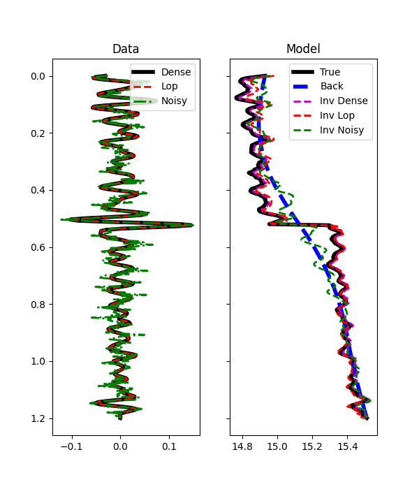
We can now estimate the acoustic profile from band-limited data using either the dense operator or linear operator.

# solve dense
minv_dense = pylops.avo.poststack.PoststackInversion(
    d, wav / 2, m0=mback, explicit=True, simultaneous=False
)[0]

# solve lop
minv = pylops.avo.poststack.PoststackInversion(
    d_dense,
    wav / 2,
    m0=mback,
    explicit=False,
    simultaneous=False,
    **dict(iter_lim=2000)
)[0]

# solve noisy
mn = pylops.avo.poststack.PoststackInversion(
    dn_dense, wav / 2, m0=mback, explicit=True, epsR=1e0, **dict(damp=1e-1)
)[0]

fig, axs = plt.subplots(1, 2, figsize=(6, 7), sharey=True)
axs[0].plot(d_dense, t0, "k", lw=4, label="Dense")
axs[0].plot(d, t0, "--r", lw=2, label="Lop")
axs[0].plot(dn_dense, t0, "-.g", lw=2, label="Noisy")
axs[0].set_title("Data")
axs[0].invert_yaxis()
axs[0].axis("tight")
axs[0].legend(loc=1)
axs[1].plot(m, t0, "k", lw=4, label="True")
axs[1].plot(mback, t0, "--b", lw=4, label="Back")
axs[1].plot(minv_dense, t0, "--m", lw=2, label="Inv Dense")
axs[1].plot(minv, t0, "--r", lw=2, label="Inv Lop")
axs[1].plot(mn, t0, "--g", lw=2, label="Inv Noisy")
axs[1].set_title("Model")
axs[1].axis("tight")
axs[1].legend(loc=1)

Out:

<matplotlib.legend.Legend object at 0x7f90d124ceb8>

We see how inverting a dense matrix is in this case faster than solving for the linear operator (a good estimate of the model is in fact obtained only after 2000 iterations of lsqr). Nevertheless, having a linear operator is useful when we deal with larger dimensions (2d or 3d) and we want to couple our modelling operator with different types of spatial regularizations or preconditioning.

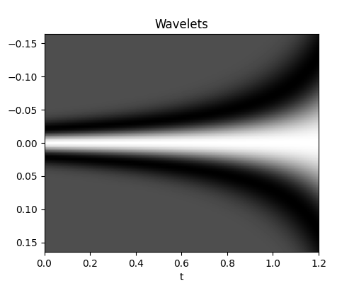
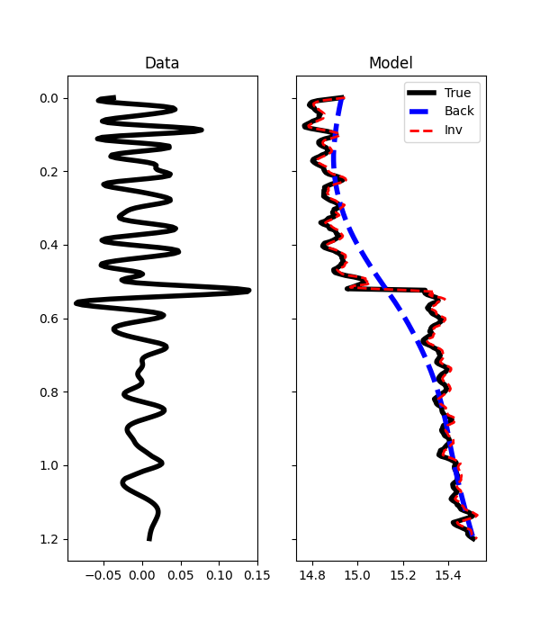
Before we move onto a 2d example, let’s consider the case of non-stationary wavelet and see how we can easily use the same routines in this case

# wavelet
ntwav = 41
f0s = np.flip(np.arange(nt0) * 0.05 + 3)
wavs = np.array([ricker(t0[:ntwav], f0)[0] for f0 in f0s])
wavc = np.argmax(wavs[0])

plt.figure(figsize=(5, 4))
plt.imshow(wavs.T, cmap="gray", extent=(t0[0], t0[-1], t0[ntwav], -t0[ntwav]))
plt.xlabel("t")
plt.title("Wavelets")
plt.axis("tight")

# operator
PPop = pylops.avo.poststack.PoststackLinearModelling(wavs / 2, nt0=nt0, explicit=True)

# data
d = PPop * m

# solve
minv = pylops.avo.poststack.PoststackInversion(
    d, wavs / 2, m0=mback, explicit=True, **dict(cond=1e-10)
)[0]

fig, axs = plt.subplots(1, 2, figsize=(6, 7), sharey=True)
axs[0].plot(d, t0, "k", lw=4)
axs[0].set_title("Data")
axs[0].invert_yaxis()
axs[0].axis("tight")
axs[1].plot(m, t0, "k", lw=4, label="True")
axs[1].plot(mback, t0, "--b", lw=4, label="Back")
axs[1].plot(minv, t0, "--r", lw=2, label="Inv")
axs[1].set_title("Model")
axs[1].axis("tight")
axs[1].legend(loc=1)

• 
• 

Out:

<matplotlib.legend.Legend object at 0x7f90cd6e10b8>

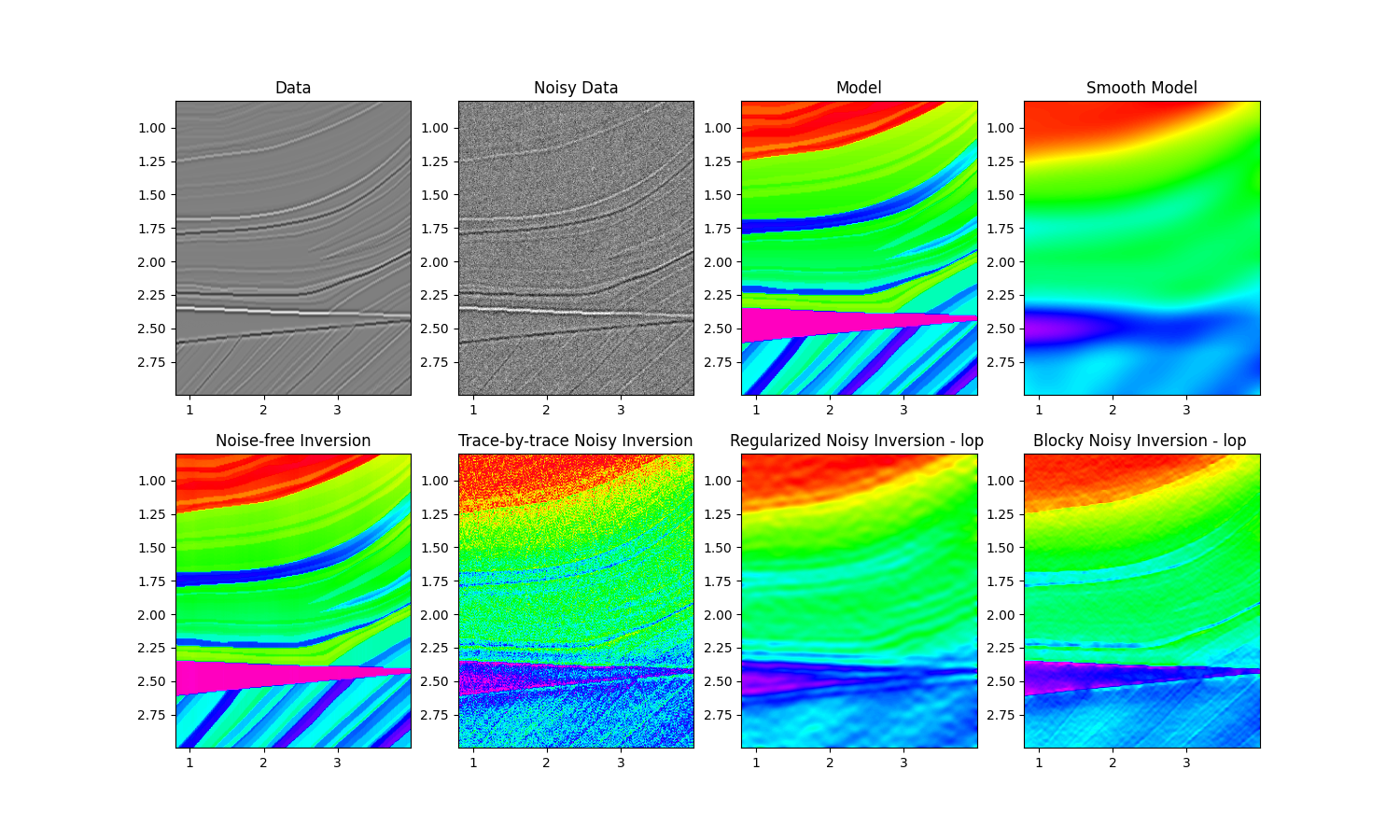
We move now to a 2d example. First of all the model is loaded and data generated.

# model
inputfile = "../testdata/avo/poststack_model.npz"

model = np.load(inputfile)
m = np.log(model["model"][:, ::3])
x, z = model["x"][::3] / 1000.0, model["z"] / 1000.0
nx, nz = len(x), len(z)

# smooth model
nsmoothz, nsmoothx = 60, 50
mback = filtfilt(np.ones(nsmoothz) / float(nsmoothz), 1, m, axis=0)
mback = filtfilt(np.ones(nsmoothx) / float(nsmoothx), 1, mback, axis=1)

# dense operator
PPop_dense = pylops.avo.poststack.PoststackLinearModelling(
    wav / 2, nt0=nz, spatdims=nx, explicit=True
)

# lop operator
PPop = pylops.avo.poststack.PoststackLinearModelling(wav / 2, nt0=nz, spatdims=nx)

# data
d = (PPop_dense * m.ravel()).reshape(nz, nx)
n = np.random.normal(0, 1e-1, d.shape)
dn = d + n

Finally we perform 4 different inversions:

• trace-by-trace inversion with explicit solver and dense operator with noise-free data

• trace-by-trace inversion with explicit solver and dense operator with noisy data

• multi-trace regularized inversion with iterative solver and linear operator using the result of trace-by-trace inversion as starting guess

  \[J = ||\Delta \mathbf{d} - \mathbf{W} \Delta \mathbf{ai}||_2 + \epsilon_\nabla ^2 ||\nabla \mathbf{ai}||_2\]

  where \(\Delta \mathbf{d}=\mathbf{d}-\mathbf{W}\mathbf{AI_0}\) is the residual data

• multi-trace blocky inversion with iterative solver and linear operator

# dense inversion with noise-free data
minv_dense = pylops.avo.poststack.PoststackInversion(
    d, wav / 2, m0=mback, explicit=True, simultaneous=False
)[0]

# dense inversion with noisy data
minv_dense_noisy = pylops.avo.poststack.PoststackInversion(
    dn, wav / 2, m0=mback, explicit=True, epsI=4e-2, simultaneous=False
)[0]

# spatially regularized lop inversion with noisy data
minv_lop_reg = pylops.avo.poststack.PoststackInversion(
    dn,
    wav / 2,
    m0=minv_dense_noisy,
    explicit=False,
    epsR=5e1,
    **dict(damp=np.sqrt(1e-4), iter_lim=80)
)[0]

# blockiness promoting inversion with noisy data
minv_lop_blocky = pylops.avo.poststack.PoststackInversion(
    dn,
    wav / 2,
    m0=mback,
    explicit=False,
    epsR=[0.4],
    epsRL1=[0.1],
    **dict(mu=0.1, niter_outer=5, niter_inner=10, iter_lim=5, damp=1e-3)
)[0]

fig, axs = plt.subplots(2, 4, figsize=(15, 9))
axs[0][0].imshow(d, cmap="gray", extent=(x[0], x[-1], z[-1], z[0]), vmin=-0.4, vmax=0.4)
axs[0][0].set_title("Data")
axs[0][0].axis("tight")
axs[0][1].imshow(
    dn, cmap="gray", extent=(x[0], x[-1], z[-1], z[0]), vmin=-0.4, vmax=0.4
)
axs[0][1].set_title("Noisy Data")
axs[0][1].axis("tight")
axs[0][2].imshow(
    m,
    cmap="gist_rainbow",
    extent=(x[0], x[-1], z[-1], z[0]),
    vmin=m.min(),
    vmax=m.max(),
)
axs[0][2].set_title("Model")
axs[0][2].axis("tight")
axs[0][3].imshow(
    mback,
    cmap="gist_rainbow",
    extent=(x[0], x[-1], z[-1], z[0]),
    vmin=m.min(),
    vmax=m.max(),
)
axs[0][3].set_title("Smooth Model")
axs[0][3].axis("tight")
axs[1][0].imshow(
    minv_dense,
    cmap="gist_rainbow",
    extent=(x[0], x[-1], z[-1], z[0]),
    vmin=m.min(),
    vmax=m.max(),
)
axs[1][0].set_title("Noise-free Inversion")
axs[1][0].axis("tight")
axs[1][1].imshow(
    minv_dense_noisy,
    cmap="gist_rainbow",
    extent=(x[0], x[-1], z[-1], z[0]),
    vmin=m.min(),
    vmax=m.max(),
)
axs[1][1].set_title("Trace-by-trace Noisy Inversion")
axs[1][1].axis("tight")
axs[1][2].imshow(
    minv_lop_reg,
    cmap="gist_rainbow",
    extent=(x[0], x[-1], z[-1], z[0]),
    vmin=m.min(),
    vmax=m.max(),
)
axs[1][2].set_title("Regularized Noisy Inversion - lop ")
axs[1][2].axis("tight")
axs[1][3].imshow(
    minv_lop_blocky,
    cmap="gist_rainbow",
    extent=(x[0], x[-1], z[-1], z[0]),
    vmin=m.min(),
    vmax=m.max(),
)
axs[1][3].set_title("Blocky Noisy Inversion - lop ")
axs[1][3].axis("tight")

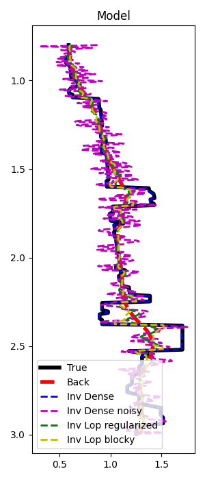
fig, ax = plt.subplots(1, 1, figsize=(3, 7))
ax.plot(m[:, nx // 2], z, "k", lw=4, label="True")
ax.plot(mback[:, nx // 2], z, "--r", lw=4, label="Back")
ax.plot(minv_dense[:, nx // 2], z, "--b", lw=2, label="Inv Dense")
ax.plot(minv_dense_noisy[:, nx // 2], z, "--m", lw=2, label="Inv Dense noisy")
ax.plot(minv_lop_reg[:, nx // 2], z, "--g", lw=2, label="Inv Lop regularized")
ax.plot(minv_lop_blocky[:, nx // 2], z, "--y", lw=2, label="Inv Lop blocky")
ax.set_title("Model")
ax.invert_yaxis()
ax.axis("tight")
ax.legend()
plt.tight_layout()

• 
• 

That’s almost it. If you wonder how this can be applied to real data, head over to the following notebook where the open-source segyio library is used alongside pylops to create an end-to-end open-source seismic inversion workflow with SEG-Y input data.