AVO modelling

This example shows how to create pre-stack angle gathers using the pylops.avo.avo.AVOLinearModelling operator.

import matplotlib.pyplot as plt
import numpy as np
from scipy.signal import filtfilt

import pylops
from pylops.utils.wavelets import ricker

plt.close("all")
np.random.seed(0)

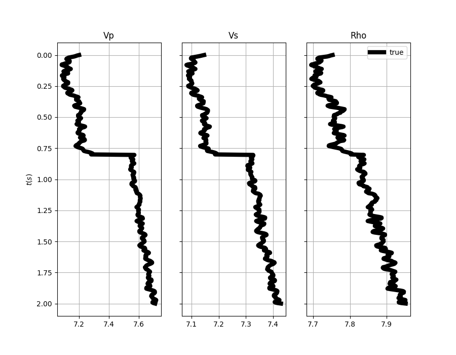
Let’s start by creating the input elastic property profiles

nt0 = 501
dt0 = 0.004
ntheta = 21

t0 = np.arange(nt0) * dt0
thetamin, thetamax = 0, 40
theta = np.linspace(thetamin, thetamax, ntheta)

# Elastic property profiles
vp = 1200 + np.arange(nt0) + filtfilt(np.ones(5) / 5.0, 1, np.random.normal(0, 80, nt0))
vs = 600 + vp / 2 + filtfilt(np.ones(5) / 5.0, 1, np.random.normal(0, 20, nt0))
rho = 1000 + vp + filtfilt(np.ones(5) / 5.0, 1, np.random.normal(0, 30, nt0))
vp[201:] += 500
vs[201:] += 200
rho[201:] += 100

# Wavelet
ntwav = 41
wavoff = 10
wav, twav, wavc = ricker(t0[: ntwav // 2 + 1], 20)
wav_phase = np.hstack((wav[wavoff:], np.zeros(wavoff)))

# vs/vp profile
vsvp = 0.5
vsvp_z = np.linspace(0.4, 0.6, nt0)

# Model
m = np.stack((np.log(vp), np.log(vs), np.log(rho)), axis=1)

fig, axs = plt.subplots(1, 3, figsize=(9, 7), sharey=True)
axs[0].plot(m[:, 0], t0, "k", lw=6)
axs[0].set_title("Vp")
axs[0].set_ylabel(r"$t(s)$")
axs[0].invert_yaxis()
axs[0].grid()
axs[1].plot(m[:, 1], t0, "k", lw=6)
axs[1].set_title("Vs")
axs[1].invert_yaxis()
axs[1].grid()
axs[2].plot(m[:, 2], t0, "k", lw=6, label="true")
axs[2].set_title("Rho")
axs[2].invert_yaxis()
axs[2].grid()
axs[2].legend()

Out:

<matplotlib.legend.Legend object at 0x7f90d0ff4940>

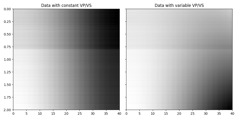
We create now the operators to model the AVO responses for a set of elastic profiles

# constant vsvp
PPop_const = pylops.avo.avo.AVOLinearModelling(
    theta, vsvp=vsvp, nt0=nt0, linearization="akirich", dtype=np.float64
)

# depth-variant vsvp
PPop_variant = pylops.avo.avo.AVOLinearModelling(
    theta, vsvp=vsvp_z, linearization="akirich", dtype=np.float64
)

We can then apply those operators to the elastic model and create some synthetic reflection responses

dPP_const = PPop_const * m.ravel()
dPP_const = dPP_const.reshape(nt0, ntheta)

dPP_variant = PPop_variant * m.ravel()
dPP_variant = dPP_variant.reshape(nt0, ntheta)

fig, axs = plt.subplots(1, 2, figsize=(10, 5), sharey=True)
axs[0].imshow(
    dPP_const,
    cmap="gray",
    extent=(theta[0], theta[-1], t0[-1], t0[0]),
    vmin=dPP_const.min(),
    vmax=dPP_const.max(),
)
axs[0].set_title("Data with constant VP/VS")
axs[0].axis("tight")
axs[1].imshow(
    dPP_variant,
    cmap="gray",
    extent=(theta[0], theta[-1], t0[-1], t0[0]),
    vmin=dPP_variant.min(),
    vmax=dPP_variant.max(),
)
axs[1].set_title("Data with variable VP/VS")
axs[1].axis("tight")
plt.tight_layout()

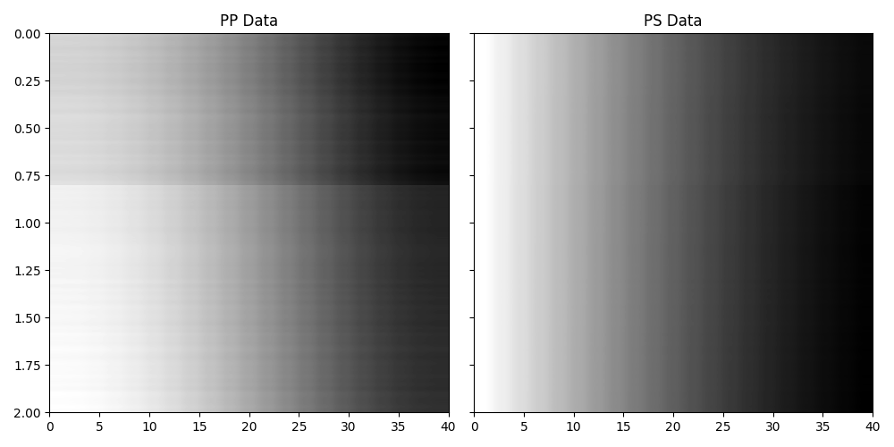
Finally we can also model the PS response by simply changing the linearization choice as follows

PSop = pylops.avo.avo.AVOLinearModelling(
    theta, vsvp=vsvp, nt0=nt0, linearization="ps", dtype=np.float64
)

We can then apply those operators to the elastic model and create some synthetic reflection responses

dPS = PSop * m.ravel()
dPS = dPS.reshape(nt0, ntheta)

fig, axs = plt.subplots(1, 2, figsize=(10, 5), sharey=True)
axs[0].imshow(
    dPP_const,
    cmap="gray",
    extent=(theta[0], theta[-1], t0[-1], t0[0]),
    vmin=dPP_const.min(),
    vmax=dPP_const.max(),
)
axs[0].set_title("PP Data")
axs[0].axis("tight")
axs[1].imshow(
    dPS,
    cmap="gray",
    extent=(theta[0], theta[-1], t0[-1], t0[0]),
    vmin=dPS.min(),
    vmax=dPS.max(),
)
axs[1].set_title("PS Data")
axs[1].axis("tight")
plt.tight_layout()