Bilinear Interpolation

This example shows how to use the pylops.signalprocessing.Bilinar operator to perform bilinear interpolation to a 2-dimensional input vector.

import matplotlib.gridspec as pltgs
import matplotlib.pyplot as plt
import numpy as np
from scipy import misc

import pylops

plt.close("all")
np.random.seed(0)

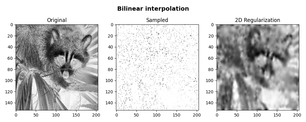
First of all, we create a 2-dimensional input vector containing an image from the scipy.misc family.

x = misc.face()[::5, ::5, 0]
nz, nx = x.shape

We can now define a set of available samples in the first and second direction of the array and apply bilinear interpolation.

nsamples = 2000
iava = np.vstack(
    (np.random.uniform(0, nz - 1, nsamples), np.random.uniform(0, nx - 1, nsamples))
)

Bop = pylops.signalprocessing.Bilinear(iava, (nz, nx))
y = Bop * x.ravel()

At this point we try to reconstruct the input signal imposing a smooth solution by means of a regularization term that minimizes the Laplacian of the solution.

D2op = pylops.Laplacian((nz, nx), weights=(1, 1), dtype="float64")

xadj = Bop.H * y
xinv = pylops.optimization.leastsquares.NormalEquationsInversion(
    Bop, [D2op], y, epsRs=[np.sqrt(0.1)], returninfo=False, **dict(maxiter=100)
)
xadj = xadj.reshape(nz, nx)
xinv = xinv.reshape(nz, nx)

fig, axs = plt.subplots(1, 3, figsize=(10, 4))
fig.suptitle("Bilinear interpolation", fontsize=14, fontweight="bold", y=0.95)
axs[0].imshow(x, cmap="gray_r", vmin=0, vmax=250)
axs[0].axis("tight")
axs[0].set_title("Original")
axs[1].imshow(xadj, cmap="gray_r", vmin=0, vmax=250)
axs[1].axis("tight")
axs[1].set_title("Sampled")
axs[2].imshow(xinv, cmap="gray_r", vmin=0, vmax=250)
axs[2].axis("tight")
axs[2].set_title("2D Regularization")
plt.tight_layout()
plt.subplots_adjust(top=0.8)